Chapter 10 - Markov Chain Monte Carlo: Exercise solutions

Author

Mattias Villani

Click on the arrow to see a solution.

Exercise 10.1

This exercise extends the analysis of the Weibull model for survival times of lung cancer patients in Exercise to the regression setting. The survival times are here modelled as independent Weibull distributed with a scale parameter \(\lambda\) that is a function of covariates, i.e. using a Weibull regression model. The response variable time is denoted by \(y\) and is modelled as a function of the three covariates age, sex and ph.ecog (ECOG performance score). The model for patient \(i\) is: \[ y_i \vert \mathbf{x}_i, \boldsymbol{\beta}, k \overset{\mathrm{ind}}{\sim} \mathrm{Weibull}\big(\lambda_i = \exp(\mathbf{x}_i^\top \boldsymbol{\beta}),k\big). \] where \(\boldsymbol{\beta}\) is the vector with regression coefficients. Note that by the properties of the Weibull distribution, the conditional mean in this model is \(\mathbb{E}(y \vert \mathbf{x}_i) = \lambda_i\Gamma(1+1/k)\), so the regression coefficients do not quite have the usual interpretation of the effect on the conditional mean. The three covariates are placed in a \(n\times p\) matrix \(\mathbf{X}\) with the first column being one for all observations to model the intercept. Use a multivariate normal prior for \(\boldsymbol{\beta} \sim N(\mathbf{0},\tau^2\mathbf{I}_p)\) with the non-informative choice \(\tau = 100\), and the prior \(\ k \sim \mathrm{logNormal}(0,2^2)\). Remove the patients with missing values in the selected covariates.

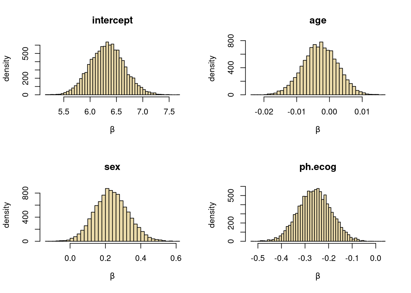
Sample from the posterior distribution \(p(\boldsymbol{\beta}, k \vert \mathbf{y}, \mathbf{X})\) using HMC in stan. Plot the marginal posterior for \(k\) and the marginal posteriors of each regression coefficient.

Solution

library(tidyverse) # loads data manipulation and visualization packages
library(rstan)
colors = c("#6C8EBF", "#c0a34d", "#780000","#007878","#B5C6DF","#EADAAA","#AE6666")

The code below defines the iid Weibull survival model with censored data in stan. The code here extends this example in the Stan User Guide to the case with different censoring points for each patient. Note the target += construction where the censored data points are added to the target (the log posterior) after the initial uncensored (observed) data are included in the log posterior with the y_obs ~ weibull(k, lambda) statement. The weibull_lccdf function in stan is a convenience function that computes the survival probability \(\mathrm{Pr}(X >= x) = 1 - F(x)\), where \(F()\) is the cdf of the Weibull distribution. There are _lccdf versions of all distribution in stan.

weibull_survivalmodel <- '
data {

  // Data
  int<lower=0> N_obs;
  int<lower=0> N_cens;
  array[N_obs] real y_obs;
  array[N_cens] real y_cens;
  
  // Model setting
  real<lower=0> k;
  
  // Prior hyperparameters theta ~ Gamma(alpha, beta)
  real<lower=0> alpha;
  real<lower=0> beta;
}
parameters {
  real lambda;
}
model {
  lambda ~ gamma(alpha, beta); // specifies the prior
  y_obs ~ weibull(k, lambda);  // add the observed (non-censored) data
  target += weibull_lccdf(y_cens | k, lambda); // add censored. lccdf is 1-cdf
}
'

We set up the data and prior lists that will be supplied to stan:

library(survival) # loads the lung cancer data as `lung`
k = 3/2
y_obs <- lung %>% filter(status == 2) %>% pull(time)
y_cens <- lung %>% filter(status == 1) %>% pull(time)

data <- list(N_obs = length(y_obs), N_cens = length(y_cens), 
             y_obs = y_obs, y_cens = y_cens, k = k)

alpha_prior <- 3     # shape parameter
beta_prior <- 1/50   # rate parameter
prior <- list(alpha = alpha_prior, beta = beta_prior)

Load rstan and set some options

#install.packages("rstan", repos = c('https://stan-dev.r-universe.dev', 
#                                    getOption("repos")))
suppressMessages(library(rstan))
options(mc.cores = parallel::detectCores())
rstan_options(auto_write = TRUE)

Sample from the posterior distribution using HMC in stan

nDraws = 5000
fit = stan(model_code = weibull_survivalmodel, data = c(data, prior), iter = nDraws)

Exercise 10.2

Exercise plotted the posterior for the parameter \(\lambda\) in the Weibull model \[ X_1,\ldots,X_n \vert \lambda, k \overset{\mathrm{iid}}{\sim} \mathrm{Weibull}(\lambda,k). \] for different fixed values of \(k\). This exercise asks you to implement the same model in to sample from the posterior distribution of \(\lambda\) for a given \(k=3/2\). The describes how to implement censoring in the model. The example in the User Guide has the same censoring point for all patients, which is not the case in the dataset. So you need to generalize that to a vector of censoring points, one for each patient.

Solution

library(tidyverse) # loads data manipulation and visualization packages
library(rstan)
colors = c("#6C8EBF", "#c0a34d", "#780000","#007878","#B5C6DF","#EADAAA","#AE6666")

Set data and set up prior hyperparameters

library(survival) # loads the lung cancer data as `lung`
lung <- lung %>% select(c("time", "status", "age", "sex", "ph.ecog")) %>% drop_na()
y = lung$time
X = cbind(1, lung$age, lung$sex == 2, lung$ph.ecog) # sex = 1 is female
p = dim(X)[2]
censored = (lung$status == 1)
y_obs = y[-censored]
y_cens = y[censored]
X_obs = X[-censored,]
X_cens = X[censored,]
mu <- rep(0,p)  # beta ~ N(mu, tau^2*I)
tau <- 100    
mu_k <- 0       # k ~ LogNormal(mu_k, sigma_k^2)
sigma_k <- 2

Set up the stan model for the Weibull regression.

weibull_survivalreg <- '
data {

  // Data
  int<lower=0> N_obs;
  int<lower=0> N_cens;
  int<lower=1> p;
  array[N_obs] real y_obs;
  array[N_cens] real y_cens;
  matrix[N_obs,p] X_obs;
  matrix[N_cens,p] X_cens;
  
  // Prior hyperparameters k ~ LogNormal(mu_k, sigma_k) and beta_ ~ N(0, tau^2*I)
  real mu_k;
  real<lower=0> sigma_k;
  real<lower = 0> tau;
}
parameters {
  vector[p] beta_;
  real<lower=0> k;
}
model {
  k ~ lognormal(mu_k, sigma_k);    // specifies the prior
  beta_ ~ normal(0, tau);
  y_obs ~ weibull(k, exp(X_obs * beta_));  // add the observed (non-censored) data
  target += weibull_lccdf(y_cens | k, exp(X_cens * beta_)); // add censored. 
}
'

We set up the data and prior lists that will be supplied to stan:

data <- list(p = dim(X_obs)[2], N_obs = length(y_obs), N_cens = length(y_cens), 
             y_obs = y_obs, y_cens = y_cens, X_obs = X_obs, X_cens = X_cens)

prior <- list(tau = tau, mu_k = mu_k, sigma_k = sigma_k)

Load rstan and set some options

#install.packages("rstan", repos = c('https://stan-dev.r-universe.dev', 
#                                    getOption("repos")))
suppressMessages(library(rstan))
options(mc.cores = parallel::detectCores())
rstan_options(auto_write = TRUE)

Sample from the posterior distribution using HMC in stan

nDraws = 5000
fit = stan(model_code = weibull_survivalreg, data = c(data, prior), iter = nDraws)

s <- summary(fit, pars = c("beta_", "k"), probs = c(0.025, 0.975))
s$summary  # results from all the different runs (chains) merged.

                 mean      se_mean          sd        2.5%        97.5%
beta_[1]  6.326162394 4.869551e-03 0.323775649  5.70127222  6.968225881
beta_[2] -0.002834145 7.845797e-05 0.005254269 -0.01319023  0.007348398
beta_[3]  0.234288159 1.080355e-03 0.095184244  0.05184712  0.425373285
beta_[4] -0.259055417 8.814885e-04 0.069571466 -0.39388588 -0.124469559
k         1.449843839 8.886235e-04 0.074705666  1.30512775  1.599808428
            n_eff     Rhat
beta_[1] 4420.898 1.001538
beta_[2] 4484.877 1.001563
beta_[3] 7762.421 1.000146
beta_[4] 6229.154 1.000016
k        7067.592 1.000660

Plotting the marginal posterior of \(k\)

# Plot histogram from stan draws
postsamples <- extract(fit, pars = c("beta_","k"))
hist(postsamples$k, 50, freq = FALSE, col = colors[5], 
     xlab = expression(k), ylab = "posterior density", 
     main = expression(k))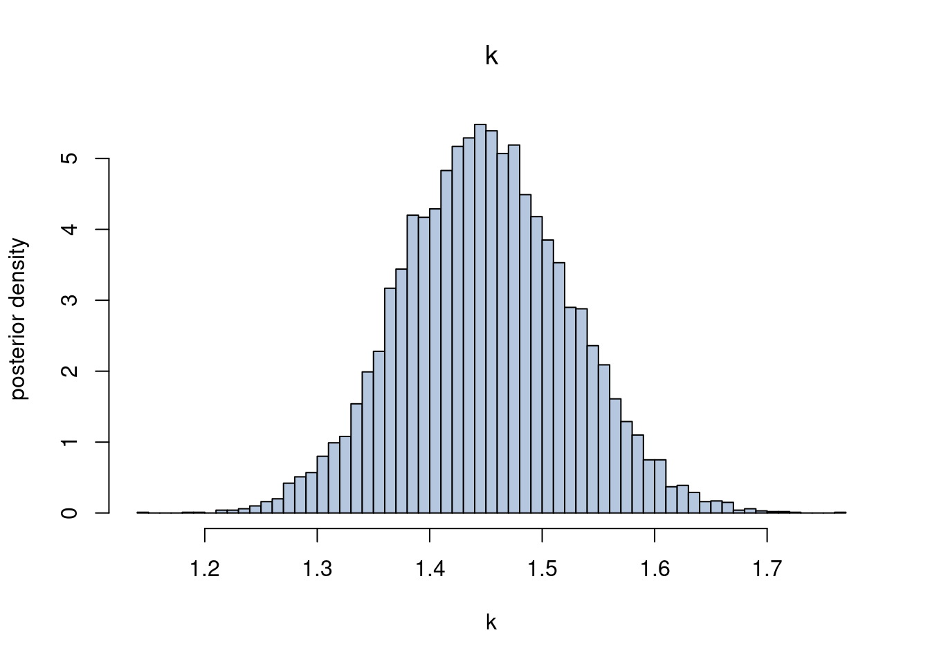

Plotting the marginal posteriors for each \(\beta\) coefficient

varNames = c("intercept", "age", "sex", "ph.ecog")
par(mfrow = c(2,2))
for (j in 1:p){
  hist(postsamples$beta_[,j], 50, col = colors[6], 
       xlab = expression(beta), ylab = "density", main = varNames[j])
}