library(tidyverse) # loads data manipulation and visualization packages
library(survival) # loads the lung cancer data as `lung`
colors = c("#6C8EBF", "#c0a34d", "#780000","#007878","#B5C6DF","#EADAAA","#AE6666")Chapter 2 - Single-parameter models: Exercise solutions
Click on the arrow to see a solution.
Exercise 2.1
Let \(X_1,\ldots,X_n \vert \theta \overset{\mathrm{iid}}{\sim} \mathrm{Expon}(\theta)\) be iid exponentially distributed data. Show that the Gamma distribution is the conjugate prior for this model.
Exercise 2.2
The dataset \(\texttt{lung}\) in the R package \(\texttt{survival}\) contains data on 228 patients with advanced lung cancer. We will here analyze the survival time of the patient in days (\(\texttt{time}\)). The variable \(\texttt{status}\) is a binary variable with \(\texttt{status}=1\) if the survival time of the patient is censored (patient was still alive at the end of the study) and \(\texttt{status}=2\) if the survival time was uncensored (patient was dead before the end of the study).
In this exercise we will only analyze the uncensored patients; Exercise below asks you to analyze all patients. Assume that the survival times \(X_1,\ldots,X_n\) of the uncensored patients are iid \(\mathrm{Expon}(\theta)\) distributed. Use the conjugate prior \(\theta \sim \mathrm{Gamma}(\alpha=3,\beta=300)\), which can be shown to imply that the expected survival time \(\mathbb{E}(X \vert \theta) = 1/\theta\) for this population is around \(200\) days. Plot the prior and posterior densities for \(\theta\) over a suitable grid of \(\theta\)-values.
Solution
From Exercise 2.1, we know that the posterior distribution is \[\theta \sim \mathrm{Gamma}(\alpha + n_u, \beta + \sum\nolimits_{u \in \mathcal{U}} x_u),\] where \(n_u\) is the number of uncensored observations and \(\mathcal{U}\) is the set of observation indices for the uncensored data.
The following code plots the prior, likelihood (normalized) and posterior over a grid of values for \(\theta\). Note that the data is so much stronger than the prior that the posterior is virtually identical to the likelihood, which is why the normalized likelihood is not visible in the plot.
# Summarize the data needed for the posterior, filter out censored data
data_summary <- lung %>% filter(status == 2) %>% summarize(n = n(), sum_x = sum(time))
# Set up prior hyperparameters
alpha_prior <- 3 # shape parameter
beta_prior <- 300 # rate parameter
# Compute posterior hyperparameters
alpha_post <- alpha_prior + data_summary$n
beta_post <- beta_prior + data_summary$sum_x # Plot the prior and posterior densities, and the (normalized) likelihood
thetaGrid <- seq(0, 0.03, length.out = 1000)
prior_density <- dgamma(thetaGrid, shape = alpha_prior, rate = beta_prior)
likelihood_density <- dgamma(thetaGrid, shape = data_summary$n, rate = data_summary$sum_x)
posterior_density <- dgamma(thetaGrid, shape = alpha_post, rate = beta_post)
df <- data.frame(
thetaGrid = thetaGrid,
prior = prior_density,
likelihood = likelihood_density,
posterior = posterior_density
)
df_long <- df %>% pivot_longer(-thetaGrid, names_to = "density_type", values_to = "density")
# Plot using ggplot2
ggplot(df_long) +
aes(x = thetaGrid, y = density, color = density_type) +
geom_line() +
scale_colour_manual(
breaks = c("prior", "likelihood", "posterior"),
values = c(colors[2], colors[1], colors[3])) +
labs(title = "Survival lung cancer - uncensored patients", x = expression(theta), y = "Density", color = "") +
theme_minimal()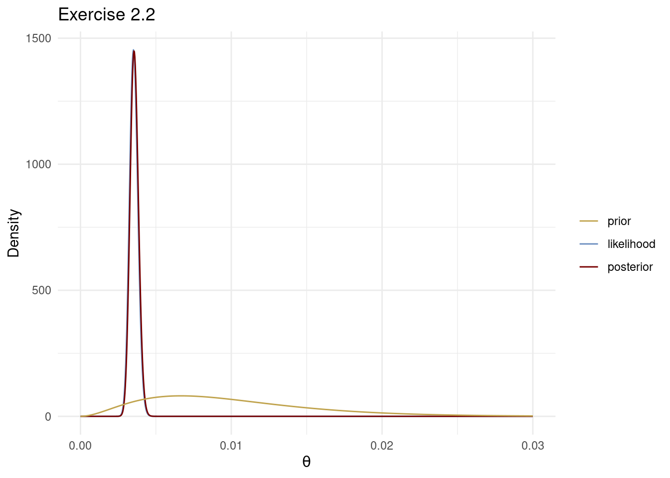
Exercise 2.3
Let \(X_1,\ldots,X_n \vert \theta \overset{\mathrm{iid}}{\sim} \mathrm{Geom}(\theta)\) be iid from a geometric distribution with parameter \(0<\theta<1\). Show that the Beta distribution is the conjugate prior for this model.
Exercise 2.4
Let \(X_1,\ldots,X_n\) be an iid sample from a distribution with density function \[ p(x) \propto \theta^2 x \exp (-x\theta)\quad \text{ for } x>0 \text{ and } \theta>0. \] Find the conjugate prior for this distribution and derive the posterior distribution from an iid sample \(x_1,\ldots,x_n\).
Exercise 2.5
a) Let \(x_{1},\ldots,x_{10}\) be a sample with mean \(\bar{x}=1.873\). Assume the model \(X_1,\ldots,X_n \overset{\mathrm{iid}}{\sim} N(\theta,1)\). Use the prior \(\theta \sim N(0,5)\). Note that the second parameter of the normal distribution is a variance, not a standard deviation. Compute the posterior distribution of \(\theta\).
b) You now get hold of a second sample \(Y_1,\ldots,Y_{10} | \theta \overset{\mathrm{iid}}{\sim} N(\theta ,2)\), where \(\theta\) is the same quantity as in (a) but the measurements have a larger variance. The sample mean in this second sample is \(\bar{y}=0.582\). Compute the posterior distribution of \(\theta\) using both samples (the \(x\)’s and the \(y\)’s) under the assumption that the two samples are independent.
\(\textit{Hint}\): batch learning.
c) You finally obtain a third sample \(Z_{1},\ldots,Z_{10} | \theta \overset{\mathrm{iid}}{\sim} N(\theta,3)\), with mean \(\bar{z}=1.221\). Unfortunately, the measuring device for this latter sample was defective and any measurement above \(3\) was recorded as exactly \(3\). There were two such measurements. Give an expression for the unnormalized posterior distribution (likelihood times prior) for \(\theta\) based on all three samples (\(x,y\) and \(z\)). Plot this unnormalized posterior over a grid of \(\theta\) values.
\(\textit{Hint}\): the posterior distribution is not normal anymore when the measurements are censored at \(3\).
Solution
Let us do as before, using the posterior from the first two samples (obtained in problem b) above) as the prior. The prior is therefore \(\theta\sim N\left(1.4237,\frac{5}{76}\right)\).
Let us first use these eight observations to update the posterior, and then afterwards add the information from the two measurements that where censored at \(3\). The mean of the eight measurements which were correctly recorded is \(\frac{1.221\cdot10-3\cdot 2}{8} = 0.77625\). The eight correctly recorded observations gives the following updating of the \(N\left(1.4237,\frac{5}{76}\right)\) prior: \[\begin{align*} w &=\frac{\frac{8}{3}}{\frac{8}{3}+\frac{1}{5/76}}=\frac{10}{67} \\ \mu_{n} &=\frac{10}{67}\cdot0.77625+\left(1-\frac{10}{67}\right)\cdot1.4237=1.3271 \\ \tau_{n}^{2} &=\left(\frac{8}{3}+\frac{1}{5/76}\right)^{-1}=\frac{15}{268}=0.05597. \end{align*}\] Note that most of the weight is now given to the prior, i.e. the posterior after the updates in (a) and (b). This is reasonable since the \(8\) new observations have a relatively large variance, \(\sigma^{2}=3\), and the prior at this step is based on \(20\) previous observations.
We are now ready for the final piece of information: the two censored observations. We do not know their exact values, but we know that they were equal to or larger than \(3\). This is important information which we cannot ignore. The likelihood from these two observations (let’s call them \(z_{1}\) and \(z_{2}\)) is \[\begin{align*} p(z_{1},z_{2}\vert\theta) &=\mathrm{Pr}(z_{1}\geq3\vert\theta)\mathrm{Pr}(z_{2}\geq3\vert\theta) \\ &=\Big(1-\mathrm{Pr}(z_{1}\leq 3\vert\theta)\Big) \Big(1-\mathrm{Pr}(z_{2}\leq3\vert\theta)\Big) \\ &=\left[1-\Phi\left(\frac{3-\theta}{\sqrt{3}}\right)\right]\left[1-\Phi\left(\frac{3-\theta}{\sqrt{3}}\right)\right] \\ &=\left[1-\Phi\left(\frac{3-\mu}{\sqrt{3}}\right)\right]^{2} \end{align*}\] where \(\Phi(\cdot)\) is the CDF of the \(\mathrm{N}(0,1)\) distribution. The posterior based on all \(30\) data points is now obtained by multiplying this likelihood with the prior at this stage, that is the posterior based on the first \(28\) correctly recorded data: \(N(1.3271,0.05597)\). The posterior is therefore proportional to \[\begin{equation*} \left[1-\Phi\left(\frac{3-\mu}{\sqrt{3}}\right)\right]^{2}\exp\left[-\frac{1}{2\cdot0.05597}\left(\mu-1.3271\right)^{2}\right]. \end{equation*}\]
The code below plots the prior (which is the posterior based on the \(28\) correctly recorded observations), the (normalized) likelihood from the two censored observations and the posterior based on all \(30\) data points. Note the form of the likelihood function from the two censored observations: the probability of observing them increases monotonically with \(\theta\) since all we know about these observations is that they are larger or equal to \(3\).
theta_grid = seq(0.5, 2.5, length = 1000)
bin_width = theta_grid[2] - theta_grid[1]
like = (1 - pnorm(3, theta_grid, sqrt(3)))^2
prior = dnorm(theta_grid, 1.3271, sqrt(0.05597))
post = like * prior # unnormalized
post = post / sum(post * bin_width)
like = like / sum(like * bin_width)
plot(theta_grid, prior, type = "l", col = "orange", lwd = 3, xlab = expression(theta), ylab = "density")
lines(theta_grid, like, col = "steelblue", lwd = 3)
lines(theta_grid, post, col = "indianred", lwd = 3)
legend("topleft", legend = c("Prior", "Likelihood (normalized)", "Posterior"),
       col = c("orange", "steelblue", "indianred"), lwd = 3, bty = "n")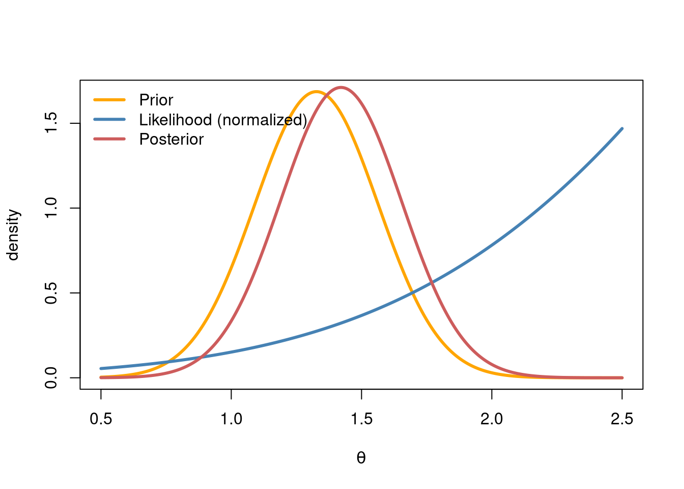
Exercise 2.6
Derive the posterior distribution for the normal model with a normal prior.
Solution

Exercise 2.7
a) Let \(X_1,\dots,X_n |\theta \sim \mathrm{Uniform}(\theta-1/2,\theta+1/2)\) for \(-\infty < \theta <\infty\). The estimator \(\hat\theta= \bar X\) is unbiased for \(\theta\). Calculate for the sampling variance of \(\hat\theta\).
\(\textit{Note}\): A more efficient estimator is the mid-range \(\hat\theta = (X_{\min} + X_{\max})/2\), but we use the sample mean here for simplicity.
b) Derive the posterior distribution for \(\theta\) assuming a uniform prior distribution over the whole real line.
\(\textit{Hint}\): once you have observed some data, some values for \(\theta\) are no longer possible.
Solution
The density for each observation in the sample is \[ p(x \vert \theta) = I\Big(\theta- \frac{1}{2} \leq x \leq \theta + \frac{1}{2}\Big). \] where \(I()\) is an indicator function that returns the value one when the condition inside the parenthesis is true, and zero otherwise. The likelihood based a single observation is therefore zero whenever \(\theta \geq x-\frac{1}{2}\) or when \(\theta \leq x + \frac{1}{2}\). So, to highlight that we care about \(p(x\vert\theta)\) as function of \(\theta\), we can write \[ p(x \vert \theta) = I\Big(x - \frac{1}{2} \leq \theta \leq x + \frac{1}{2}\Big). \]
The likelihood from an iid sample of \(n\) observation can therefore be written \[ p(x_1,\ldots,x_n \vert \theta) = \prod_{i=1}^n p(x_i \vert \theta) = \prod_{i=1}^n I\Big(x_i - \frac{1}{2} \leq \theta \leq x_i + \frac{1}{2}\Big) \] The plots below illustrate how certain \(\theta\) values makes the single data point \(x_1 = 2.1\) impossible.
Code
xi = 2.1
par(mfrow = c(3,1))

# Adding the uniform density for an impossible theta
theta = 1.2
plot(xi, 0, pch = 19, col = "indianred", xlim = c(0,4), ylim = c(-0.1,1.1),
     main = "theta = 1.2 is too low - distribution misses the data x = 2.1")
abline(h = 0, lty = "dashed")
points(theta, 0, pch = 3, col = "orange", lwd = 3)
lines(c(theta - 0.5, theta + 0.5), c(1,1), col = "orange")
lines(c(theta - 0.5, theta - 0.5), c(0,1), col = "orange")
lines(c(theta + 0.5, theta + 0.5), c(0,1), col = "orange")

# Adding the uniform density for an impossible theta
theta = 2
plot(xi, 0, pch = 19, col = "indianred", xlim = c(0,4), ylim = c(-0.1,1.1),
     main = "theta = 2 is OK - distribution captures the data x = 2.1")
abline(h = 0, lty = "dashed")
points(theta, 0, pch = 3, col = "cornflowerblue", lwd = 3)
lines(c(theta - 0.5, theta + 0.5), c(1,1), col = "cornflowerblue")
lines(c(theta - 0.5, theta - 0.5), c(0,1), col = "cornflowerblue")
lines(c(theta + 0.5, theta + 0.5), c(0,1), col = "cornflowerblue")

# Adding the uniform density for an impossible theta
theta = 3.2
plot(xi, 0, pch = 19, col = "indianred", xlim = c(0,4), ylim = c(-0.1,1.1),
     main = "theta = 3.2 is too high - distribution misses the data x = 2.1")
abline(h = 0, lty = "dashed")
points(theta, 0, pch = 3, col = "green", lwd = 3)
lines(c(theta - 0.5, theta + 0.5), c(1,1), col = "green")
lines(c(theta - 0.5, theta - 0.5), c(0,1), col = "green")
lines(c(theta + 0.5, theta + 0.5), c(0,1), col = "green")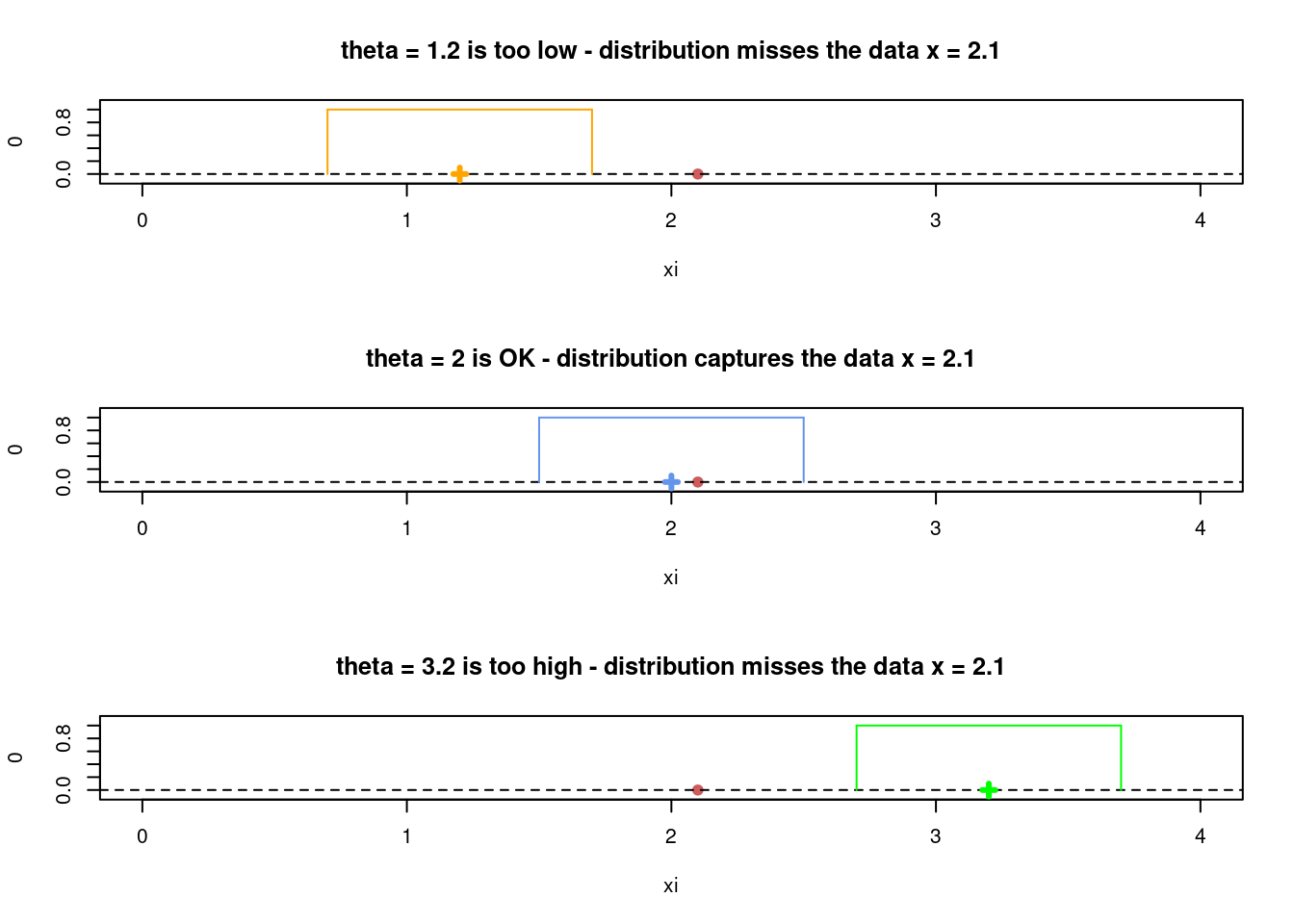
The likelihood is non-zero only for the \(\theta\) values where \(x_i - \frac{1}{2} \leq \theta \leq x_i + \frac{1}{2}\) for all data observations \(i=1,2,\ldots,n\). This means that the likelihood is non-zero only when \(x_\max - \frac{1}{2} \leq \theta \leq x_\min + \frac{1}{2}\), where \(x_\min\) and \(x_\max\) are the minimum and maximum of the sample. With a uniform prior on \(\theta\), the posterior is proportional to the likelihood, so \[ p(\theta \vert x_1,\ldots,x_n) \propto p(x_1,\ldots,x_n \vert \theta)p(\theta) \propto I\Big( x_\max - \frac{1}{2} \leq \theta \leq x_\min + \frac{1}{2} \Big) \] So the posterior distribution is \[ \theta \vert x_1,\ldots,x_n \sim \mathrm{Uniform}\Big(x_\max - \frac{1}{2} , x_\min + \frac{1}{2} \Big) \]
c) Assume that you have observed three data observations: \(x_1 = 1.1, x_2 = 2.05, x_3 = 1.21\). What would a frequentist conclude about \(\theta\)? What would a Bayesian conclude? Discuss.
Solution
The frequentist with \(\bar X\) as the estimator of \(\theta\) obtains the estimate \(\bar x \approx 1.453\). The sampling standard deviation is \(\mathbb{S}(\bar X) = \sqrt{\frac{1}{12n}} = \sqrt{\frac{1}{3\cdot 12}} \approx 0.1666\), which is the variability of the sample mean estimator on average over all possible datasets of size \(n=3\). The variability is rather large since we only have three observations, so we can easily obtain a sample with three extreme (all small or all large) observations. Here is a plot of the simulated sampling distribution for \(\bar X\) from a sample with three observations:
theta = 1  # any value is ok, it will be the center of the sampling distr.
nRep = 50000
n = 3
xbar = rep(0, nRep)
for (i in 1:nRep){
  x_rep = runif(n, min = theta - 0.5, max = theta + 0.5)
  xbar[i] = mean(x_rep)
}
hist(xbar, 50, freq = FALSE,
     main = "sampling distribution of the sample mean",
     xlab = "sample mean", ylab = "density", col = "cornflowerblue")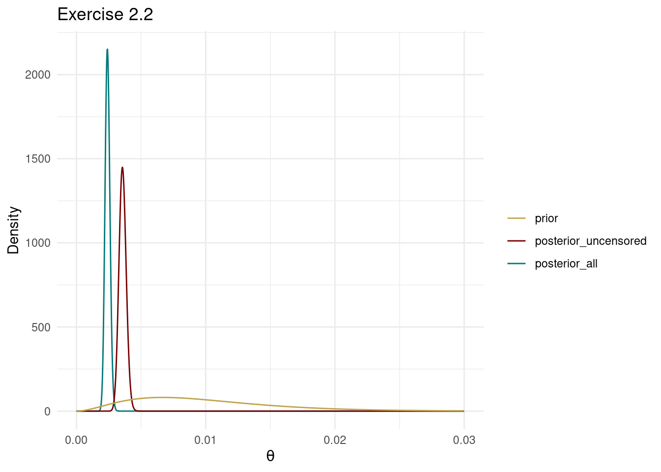
(As a side-note: note how fast the central limit theorem is here, the sampling distribution is already close to normal as \(n=3\))
For the given dataset we have \(x_\min = 1.1\) and \(x_\max = 2.05\) and the posterior is therefore \[ \theta \vert x_1,x_2,x_3 \sim \mathrm{Uniform}\big(1.55 , 1.60 \big) \] Since we were lucky to obtain a range of the data close to \(1\) (the range is the difference between the maximum and minimum observations: \(2.05-1.1 = 0.95\)), the Bayesian gets a tight posterior which is uniform between \(1.55\) and \(1.60\). The posterior is plotted here:
Code
x = c(1.10, 2.05, 1.21)
plot(x = NA, y = NA, xlim = c(1,2), ylim = c(-1,1),
     xlab = expression(theta), ylab = "posterior density")
post_low = max(x) -0.5
post_high = min(x) + 0.5
lines(c(post_low, post_high), c(1, 1), col = "orange")
lines(c(post_low, post_low), c(0, 1), col = "orange")
lines(c(post_high, post_high), c(1, 0), col = "orange")
abline(h=0, lty = "dashed")
The difference between the frequentist and Bayesian solutions is that the Bayesian solution conditions on the observed data, while the frequentist inferences are unconditional on the data, measuring the variability of the estimator over all possible datasets. We got lucky with a wide range in the actually observed data, so the Bayesian can provide a tight posterior for \(\theta\) with little uncertainty.
Exercise 2.8
Exercise modelled the survival times of uncensored lung cancer patients with an iid exponential model. In this exercise we will extend that analysis to include also the censored patients, using the same prior as in Exercise . Plot the prior and posterior densities for \(\theta\) over a suitable grid of \(\theta\)-values. Finally, assess the fit of the exponential model by plotting a histogram of \(\texttt{time}\) and overlay the pdf of the exponential model with the parameter \(\theta\) estimated with the posterior mode.
\(\textit{Hint}\): The posterior is no longer tractable due to contributions of the censored patients to the likelihood. For the censored patients we only know that they lived the number of days recorded in the dataset. The likelihood contribution \(p(x_c \vert \theta)\) for the \(c\)th censored patient with recorded time \(x_c\) is therefore \(p(X \geq x_c \vert \theta) = e^{-\theta x_c}\), which follows from the distribution function of the exponential distribution \(p(X \leq x \vert \theta) = 1 - e^{-\theta x}\).
Solution
library(tidyverse) # loads data manipulation and visualization packages
library(survival) # loads the lung cancer data as `lung`
colors = c("#6C8EBF", "#c0a34d", "#780000","#007878","#B5C6DF","#EADAAA","#AE6666")
The likelihood for all data, censored and uncensored, is \[ \begin{align} p(x_1,\ldots,x_n \vert \theta) & = \prod_{i=1}^n p(x_i \vert \theta) \\ & = \prod_{u \in \mathcal{U}} p(x_u \vert \theta) \prod_{c \in \mathcal{C}} p(x_c \vert \theta) \\ & = \prod_{u \in \mathcal{U}} p(x_u \vert \theta) \prod_{c \in \mathcal{C}} \left(1 - F(x_c \vert \theta)\right) \end{align} \] where \(\mathcal{U}\) and \(\mathcal{C}\) are the sets of observation indicies for the uncensored and censored data, respectively. The likelihood for the uncensored data (the first product) is the same as before \[ \prod_{u \in \mathcal{U}} p(x_u \vert \theta) = \prod_{u \in \mathcal{U}} \theta e^{-\theta x_u} = \theta^{n_u} e^{-\theta\sum_{u \in \mathcal{U}} x_u}, \] where \(n_u\) is the number of uncensored observations. The likelihood contribution for each observation in the censored set (the second product) is the survival function \[ \mathrm{Pr}(X \geq x_c) = 1 - F(x_c \vert \theta), \] where \(F(x_c \vert \theta) = 1 - e^{-x_c \theta}\) is the cumulative distribution function of the exponential distribution evaluated at \(x_c\).
So the likelihood function is \[ p(x_1,\ldots,x_n \vert \theta) = \theta^n e^{-\theta\sum_{u \in \mathcal{U}} x_u} \times e^{-\theta \sum_{u \in \mathcal{U}} x_c} = \theta^{n_u} e^{-\theta\sum_{i = 1}^n x_i}. \] where one should note that \(\theta\) is raised to the number of uncensored observations, \(n_u\) while the sum in the exponential term includes both uncensored and censored observations.
By Bayes’ theorem, the posterior distribution is again a Gamma distribution \[ \begin{align} p(\theta \vert x_1,\ldots,x_n) & \propto p(x_1,\ldots,x_n \vert \theta)p(\theta) \\ & \propto \theta^{n_u} e^{-\theta\sum_{i = 1}^n x_i} \times \theta^{\alpha-1}e^{-\beta\theta} \\ & = \theta^{\alpha + n_u - 1} e^{ -\theta(\beta + \sum_{i = 1}^n x_i)}, \end{align} \] which we recognize as proportional to the following Gamma distribution \[ \theta \vert x_1,\ldots,x_n \sim \mathrm{Gamma}(\alpha + n_u,\beta + \sum\nolimits_{i=1}^n x_i). \]
The code below plots both:
- the posterior from the previous exercise (a) with only the uncensored data and
- the posterior from with all data.
The posterior with all data is more informative and concentrates on smaller \(\theta\) values. Since smaller \(\theta\) values correspond to longer expected survival times, this is makes sense since the censored patients were still alive at the end of the study.
# Summarize the data needed for the posterior, grouped by `status`:
data_summary <- lung %>% group_by(status) %>% summarize(n = n(), sum_x = sum(time))
# Set up prior hyperparameters
alpha_prior <- 3 # shape parameter
beta_prior <- 300 # rate parameter
# Compute posterior hyperparameters - only uncensored data
alpha_post_u <- alpha_prior + data_summary$n[2] # second row is uncensored data (status = 2)
beta_post_u <- beta_prior + data_summary$sum_x[2] # sum over uncensored observations
# Compute posterior hyperparameters - all data
alpha_post_all <- alpha_prior + data_summary$n[2] # note: this is still n_u
beta_post_all <- beta_prior + sum(data_summary$sum_x) # sum over all observations # Plot the prior and the two posterior densities
thetaGrid <- seq(0, 0.03, length.out = 1000)
prior_density <- dgamma(thetaGrid, shape = alpha_prior, rate = beta_prior)
posterior_density_u <- dgamma(thetaGrid, shape = alpha_post_u, rate = beta_post_u)
posterior_density_all <- dgamma(thetaGrid, shape = alpha_post_all, rate = beta_post_all)
df <- data.frame(
thetaGrid = thetaGrid,
prior = prior_density,
posterior_uncensored = posterior_density_u,
posterior_all = posterior_density_all
)
df_long <- df %>% pivot_longer(-thetaGrid, names_to = "density_type", values_to = "density")
ggplot(df_long) +
aes(x = thetaGrid, y = density, color = density_type) +
geom_line() +
scale_colour_manual(
breaks = c("prior", "posterior_uncensored", "posterior_all"),
values = c(colors[2], colors[3], colors[4])) +
labs(title = "Exercise 2.2", x = expression(theta), y = "Density", color = "") +
theme_minimal()
The code below plots the histogram and the pdf of the exponential model with the parameter \(\theta\) set equal to the posterior mode. It is clear that the exponential model with its monotonically decreasing density is not fitting the data well.
postMode = df$thetaGrid[which.max(df$posterior_all)]

ggplot(lung, aes(time)) +
  geom_histogram(aes(y = after_stat(density), fill = "Data"), bins = 30) +
  stat_function(fun = dexp, args = list(rate = postMode), lwd = 1,
                aes(color = "Exponential fit"),
  ) +
  labs(title = "Exercise 2.2c - Exponential model fit to lung cancer survival", x = "days", y = "Density") +
  scale_fill_manual("", values = colors[5]) +
  scale_color_manual("", values = colors[3]) +
  theme_minimal()
Exercise 2.10
Show that the \(N(\mu,1)\) distribution belongs to the exponential family.
Solution
Exercise 2.10
Exercise modelled the survival times of uncensored lung cancer patients with an iid exponential model. Here we extend that analysis to the more general Weibull distribution: \[ X_1,\ldots,X_n \vert \lambda, k \overset{\mathrm{iid}}{\sim} \mathrm{Weibull}(\lambda,k). \] The value of \(k\) determines how the failure rate changes with time:Plot the posterior distribution of \(\lambda\) conditional on \(k=1\), \(k=3/2\) and \(k=2\). For all \(k\), use the prior \(\lambda \sim \mathrm{Gamma}(\alpha,\beta)\) with \(\alpha=3\) and \(\beta=1/50\) (which is a similar prior for \(\theta=1/\lambda\) as in Exercise 2.2). Plot the time variable as a histogram and overlay the fitted model for the three different \(k\)-values; use the posterior mode for \(\theta\) in each model when plotting the fitted model density.
\(\textit{Hint}\): the posterior distribution for \(k\neq 1\) is intractable, so use numerical evaluation of the posterior over a grid of \(\lambda\)-values.
Solution
The likelihood can be computed with separate treatment of the uncensored and censored observations: \[
\begin{align}
p(x_1,\ldots,x_n \vert \lambda, k) & = \prod_{i=1}^n p(x_i \vert \lambda, k) \\
& = \prod_{u \in \mathcal{U}} p(x_u \vert \lambda, k) \prod_{c \in \mathcal{C}} \Big(1 - F(x_c \vert \lambda, k)\Big)
\end{align}
\] where \(p(x \vert \lambda, k)\) is the pdf of a Weibull variable \[
p(x \vert \lambda, k) = \frac{k}{\lambda}\Big( \frac{x}{\lambda} \Big)^{k-1}e^{-(x/\lambda)^k}\quad\text{ for }x>0
\] which is implemented in R as dweibull. The cdf of the Weibull distribution is of rather simple form \[
F(x \vert \lambda, k) = 1 - e^{-(x/\lambda)^k}
\] and is implemented in R as pweibull.
The code below plots the prior and posterior distribution for \(\lambda\) for the three different \(k\)-values. We could have inserted the mathematical expressions for the pdf and cdf and simplified the final likelihood expression; we will instead use the dweibull and pweibull functions without simplifications since it gives a more general template that can be used for any distribution, not just the Weibull model. For numerical stability we usually compute the posterior distribution on the log scale \[
\log p(\lambda^{(j)} \vert x_1,\ldots,x_n) \propto \log p(x_1,\ldots,x_n \vert \lambda_j) + \log p(\lambda_j)
\] for a grid of equally spaced \(\lambda\)-values: \(\lambda^{(1)}\ldots,\lambda^{(J)}\). The \(\propto\) sign now means that there is a missing additive constant \(\log p(x_1,\ldots,x_n)\) which does not depend on the unknown parameter \(\lambda\). When we have computed \(\log p(\lambda \vert x_1,\ldots,x_n)\) over a grid of \(\lambda\) values we compute the posterior on the original scale by \[
p(\lambda^{(j)} \vert x_1,\ldots,x_n) \propto \exp\Big( \log p(x_1,\ldots,x_n \vert \lambda_j) + \log p(\lambda_j) \Big)
\] and then divide all numbers with the normalizing constant to make sure that the posterior integrates to one. This is done numerically by approximating the integral by a Riemann rectangle sum \[
p(\lambda^{(j)} \vert x_1,\ldots,x_n) =
\frac{\exp\Big( \log p(x_1,\ldots,x_n \vert \lambda^{(j)}) + \log p(\lambda^{(j)}) \Big)}
{\sum_{h=1}^J \exp\Big( \log p(x_1,\ldots,x_n \vert \lambda^{(h)}) + \log p(\lambda^{(h)}) \Big) \Delta}
\] where \(\Delta\) is the spacing between the grid points of \(\lambda\)-values: \(\lambda^{(1)}, \ldots, \lambda^{(J)}\).
library(tidyverse) # loads data manipulation and visualization packages
library(survival) # loads the lung cancer data as `lung`
colors = c("#6C8EBF", "#c0a34d", "#780000","#007878","#B5C6DF","#EADAAA","#AE6666")
Set up prior hyperparameters
alpha_prior <- 3     # shape parameter
beta_prior <- 1/50   # rate parameter
Set up function that computes the likelihood for any \(\lambda\) value:
# Make a function that computes the likelihood
weibull_loglike <- function(lambda, x, censored, k){
  loglik_uncensored = sum(dweibull(x[-censored], shape = k, scale = lambda,
                                   log = TRUE))
  loglik_censored = sum(pweibull(x[censored], shape = k, scale = lambda,
                                 lower.tail = FALSE, log.p = TRUE))
  return(loglik_uncensored + loglik_censored)
}
Set up a function that computes the posterior density over a grid of \(\lambda\):
weibull_posterior <- function(lambdaGrid, x, censored, k, alpha_prior, beta_prior){
  Delta = lambdaGrid[2] - lambdaGrid[1] # Grid step size
  logPrior <- dgamma(lambdaGrid, shape = alpha_prior, rate = beta_prior, log = TRUE)
  logLike <- sapply(lambdaGrid, weibull_loglike, x, censored, k)
  logPost <- logLike + logPrior
  logPost <- logPost - max(logPost) # subtract constant to avoid overflow
  post <- exp(logPost)/(sum(exp(logPost))*Delta) # original scale and normalize
  logLike <- logLike - max(logLike)
  likeNorm <- exp(logLike)/(sum(exp(logLike))*Delta) # normalized likelihood
  return(list(post = post, prior = exp(logPrior), likeNorm = likeNorm))
}
# Plot the prior and posterior densities
lambdaGrid <- seq(200, 800, length.out = 1000)
# Compute to get the prior
postRes <- weibull_posterior(lambdaGrid, lung$time, lung$status == 1, k = 1,
alpha_prior, beta_prior)
df <- data.frame(
lambdaGrid = lambdaGrid,
prior = postRes$prior
)
# Compute for all selected k values
postModes = c()
for (k in c(1, 3/2, 2)){
postRes <- weibull_posterior(lambdaGrid, lung$time, lung$status == 1, k, alpha_prior, beta_prior)
df[str_glue("posterior k={k}")] <- postRes$post
postModes = c(postModes, lambdaGrid[which.max(postRes$post)])
}
df_long <- df %>% pivot_longer(-lambdaGrid, names_to = "density_type", values_to = "density")
# Plot using ggplot2
ggplot(df_long) +
aes(x = lambdaGrid, y = density, color = density_type) +
geom_line() +
xlim(250,600) +
scale_colour_manual(
breaks = c("prior", "posterior k=1", "posterior k=1.5", "posterior k=2"),
values = c(colors[2], colors[1], colors[3], colors[4])) +
labs(title = "Exercise 2.3", x = expression(lambda), y = "Density", color = "") +
theme_minimal()Warning: Removed 1668 rows containing missing values or values outside the scale range
(`geom_line()`).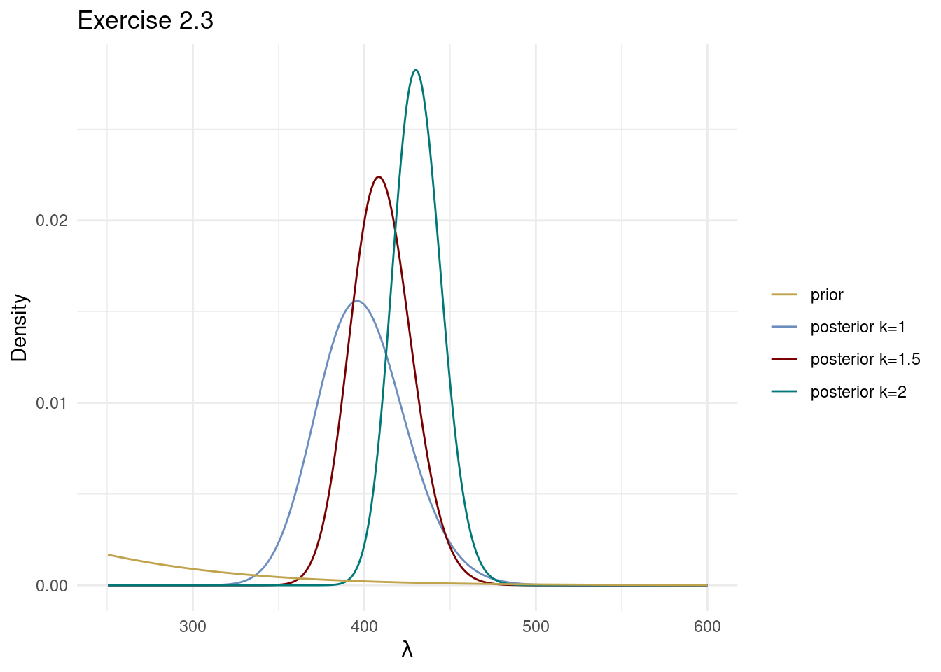
The fit of the three Weibull models are plotted below. The best fit seems to be for \(k=3/2\), but it is still not very good. In a later exercise you will be asked to freely estimate both \(\lambda\) and \(k\), and even later to fit a Weibull regression model with covariates.
ggplot(lung, aes(time)) +
  geom_histogram(aes(y = after_stat(density), fill = "Data"), bins = 30) +
  stat_function(fun = dweibull, args = list(shape = 1, scale = postModes[1]), lwd = 1,
                aes(color = "Weibull fit k = 1"),
  ) +
  stat_function(fun = dweibull, args = list(shape = 3/2, scale = postModes[2]), lwd = 1,
                aes(color = "Weibull fit k = 3/2"),
  ) +
  stat_function(fun = dweibull, args = list(shape = 2, scale = postModes[3]), lwd = 1,
                aes(color = "Weibull fit k = 2"),
  ) +
  labs(title = "Weibull model fits", x = "days", y = "Density") +
  scale_fill_manual("", values = colors[6]) +
  scale_color_manual("", values = c(colors[1], colors[3], colors[4])) +
  theme_minimal()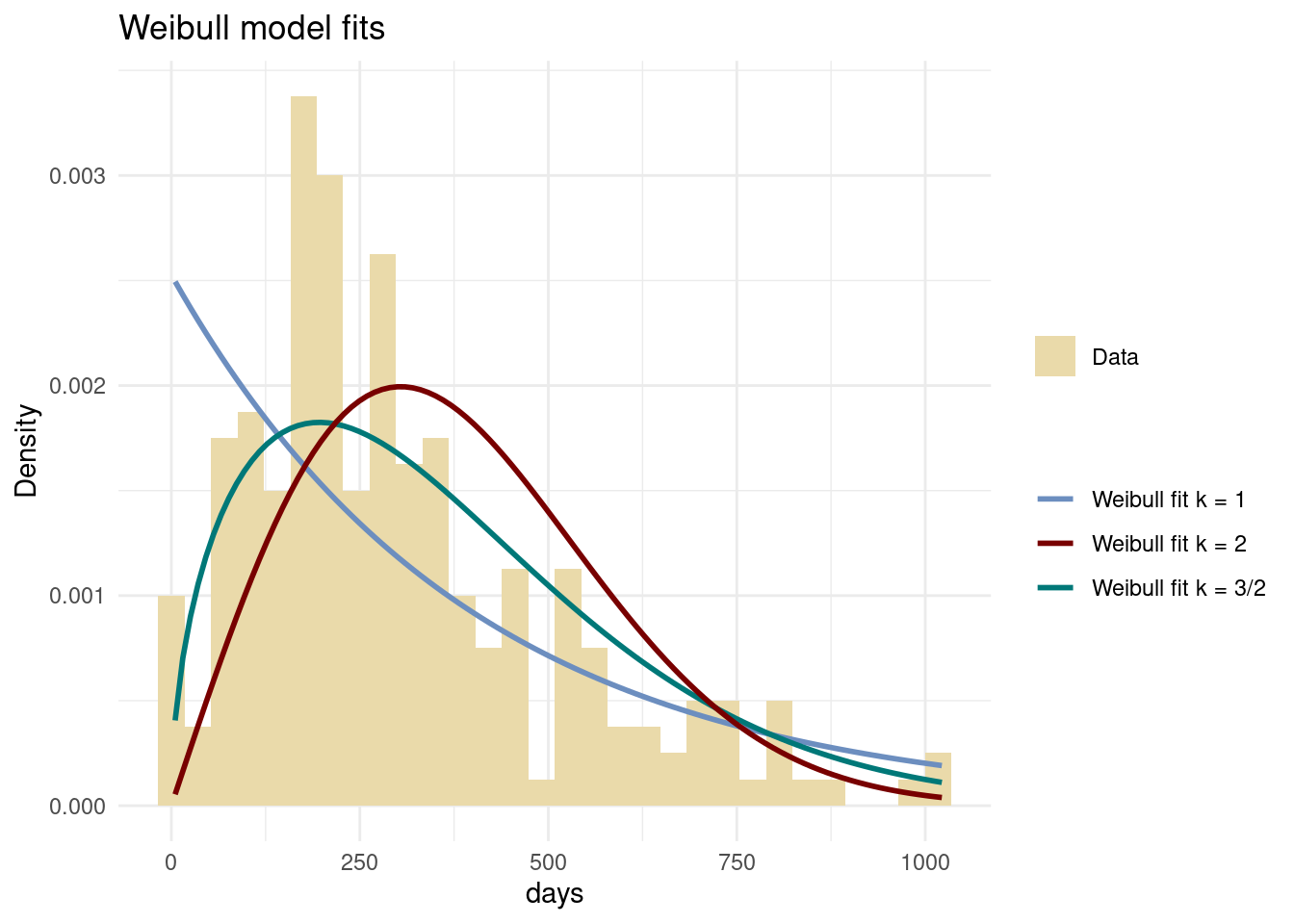
Exercise 2.11
Let \[ X_1,\ldots,X_n \overset{iid}{\sim } \mathrm{Uniform}(0,\theta). \] Show that the Pareto prior \(\theta \sim \mathrm{Pareto}(\alpha, \beta)\), is conjugate to the Uniform model by deriving the posterior distribution. See Box~ for a definition of the Pareto distribution and properties; note the support of the Pareto distribution.
\(\textit{Hint}\): Do not forget to include an indicator function when you write up the likelihood function since the \(\mathrm{Uniform}(0,\theta)\) distribution is zero for outcomes larger than \(\theta\). Also, the Pareto prior is zero for values of \(\theta < \beta\), so you need another indicator function for that.
Exercise 2.12
The number of patients per day in need of an ambulance to a small regional hospital is random following a Poisson distribution with unknown mean \(\theta\). The hospital has collected data from the past \(n=7\) days, resulting in the following daily counts of ambulance trips: \(8, 12, 6, 9, 9, 9, 5\). Before collecting the data, the head of the ambulance drivers believed that the mean number of ambulance trips per day is about \(12\) and that a mean of less than \(5\) trips is very unlikely, “like winning a lottery with only one winning ticket per hundred tickets”.
a) Compute the posterior distribution for \(\theta\) using a Gamma prior \(\theta \sim \mathrm{Gamma}(\alpha,\beta)\) with parameters \(\alpha\) and \(\beta\) set to reflect the head’s beliefs. Provide a plot of the prior distribution, the normalized likelihood and the posterior distribution.
Solution
We first need to determine the two hyperparameters \(\alpha\) and \(\beta\) of the \(\mathrm{Gamma}(\alpha,\beta)\) prior. From properties of the gamma distribution we have \[
\mathbb{E}(\theta) = \frac{\alpha}{\beta} = 12
\] to match the prior mean of the head. We must therefore have \(\alpha = 12\beta\), leaving the single hyperparameter \(\beta\) to be determined from the second condition: \[
\mathrm{Pr}(\theta < 5) = 0.01
\] Let \(F(\theta \vert \alpha,\beta)\) denote the cumulative distribution function (cdf) of the \(\mathrm{Gamma}(\alpha,\beta)\) prior. Since \(\alpha = 12\beta\) we need to solve the following equation for \(\beta\): \[
F(5 \vert 12\beta,\beta) = 0.01
\] In R code, we would like to find the beta this pgamma(5, shape = 12*beta, rate = beta) = 0.01 This cannot be (easily) solved analytically. We can either find the \(\beta\) that satisfies pgamma(5, shape = 12*beta, rate = beta) = 0.01 by trial and error (that is, try different values of beta until you get really close to pgamma(5, shape = 12*beta, rate = beta) = 0.01). A faster way is to use a numerical method (for example Newton’s method) that finds roots to equations \(f(x) = 0\) (a so called root-finding algorithm), since our problem can be formulated as finding the \(\beta\) that solves the equation \(F(5 \vert 12\beta,\beta) - 0.01 = 0\). The uniroot function in R does the job:
f <- function(x){
  return(pgamma(5, shape = 12*x, rate = x) - 0.01)
}
results = uniroot(f, c(0.001,100)) # second argument is a search interval
betaPrior = results$root
alphaPrior = 12*betaPrior
The value of \(\beta\) that satisfies the equation \(F(5 \vert 12\beta,\beta) = 0.01\) is \(\beta = 0.8472998\). We can check that this \(\beta\) indeed gives the correct prior probability \(\mathrm{Pr}(\theta < 5) = 0.01\):
pgamma(5, shape = alphaPrior, rate = betaPrior)[1] 0.01000101Bingo!
Since \(\alpha = 12\beta\), the complete prior is \(\theta \sim \mathrm{Gamma}(\alpha = 10.168, 0.847)\). Here is a plot:
thetaGrid = seq(0, 30, length = 1000)
plot(thetaGrid, dgamma(thetaGrid, shape = alphaPrior, rate = betaPrior),
     type = "l", ylab = "prior density", xlab = expression(theta),
     col = "orange", lwd = 2)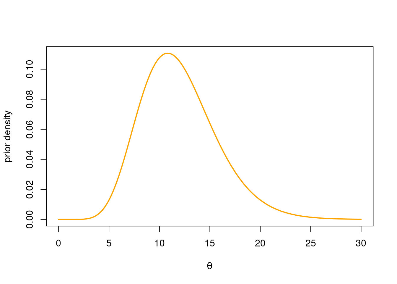
Sanity check: the mean of \(12\) seems right, and also that \(\mathrm{Pr}(\theta < 5) = 0.01\).
From Chapter 2 of the Bayesian Learning book, we know that the posterior distribution is \[ \theta \vert \boldsymbol{x} \sim \mathrm{Gamma}(\alpha + \sum_{i=1}^n x_i, \beta + n) \] So, since \(\sum_{i=1}^7 x_i = 58\) we have
x = c(8,12,6,9,9,9,5)
n = length(x)
alphaPost = alphaPrior + sum(x)
betaPost = betaPrior + n
nTheta = 1000
thetaGrid = seq(0, 15, length = nTheta)
binWidth = thetaGrid[2] - thetaGrid[1] # used to normalize likelihood
priorDens = dgamma(thetaGrid, alphaPrior, betaPrior)
postDens = dgamma(thetaGrid, alphaPost, betaPost)
like = rep(0, nTheta)
for (i in 1:nTheta){
  like[i] = prod(dpois(x, thetaGrid[i]))
}
like_norm = like/sum(binWidth*like)
plot(thetaGrid, dgamma(thetaGrid, alphaPost, betaPost),
     xlab = expression(theta), ylab = "density", type = "l",
     col = "orange", lwd = 3)
lines(thetaGrid, priorDens, col = "orange", lwd = 3)
lines(thetaGrid, like_norm, col = "steelblue", lwd = 3)
lines(thetaGrid, postDens, col = "indianred", lwd = 3)
legend("topleft", legend = c("Prior", "Likelihood (normalized)", "Posterior"),
       col = c("orange", "steelblue", "indianred"), lwd = 3, bty = "n")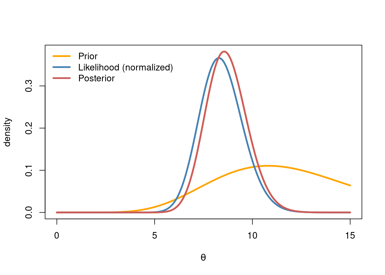
b) Compare the posterior mean, median and mode, and summarize the posterior distribution by a 95% credible interval.
Solution
Since the posterior is Gamma, we can look formulas for the mean and mode of a Gamma distribution. If \(X\sim \mathrm{Gamma}(\alpha, \beta)\), then \[ \begin{aligned} \mathbb{E}(X) &= \frac{\alpha}{\beta} \\ \mathrm{Mode}(X) &= \frac{\alpha -1}{\beta} \text{ for } \alpha \geq 1, \text{ zero otherwise} \end{aligned} \] The median is not available in closed from, but R gladly computes it with the \(qgamma\) function. Here is posterior mean, median and mode in the ambulance data example:
postMean = alphaPost/betaPost
postMedian = qgamma(0.5, alphaPost, betaPost)
postMode = (alphaPost - 1)/betaPost
message("The posterior mean is ", round(postMean,3))
The posterior mean is 8.687message("The posterior median is ", round(postMedian,3))The posterior median is 8.644message("The posterior mode is ", round(postMode,3))The posterior mode is 8.559Since the posterior distribution is fairly symmetric, these three measures of posterior location are similar.
Finally, a 95% credible interval can be computed by the following code (there are many ways of doing this). The code assumes for simplicity that the HPD interval is truly an interval, and not several disjoint intervals, as would happen when the posterior is multimodal. We know from the plot above that the posterior is unimodal, so the code is safe to use here.
# first, sort the density values from highest to lowest
postDensOrdered = sort(postDens, decreasing = TRUE)
# reorder the thetaValues so that they still match the density values
thetaOrdered = thetaGrid[order(postDens, decreasing = TRUE)]
cumsumPostDens = cumsum(binWidth*postDensOrdered) # posterior cdf
inHPD = which(cumsumPostDens < 0.95) # find highest pdf vals up to 95% quota.
hpd = c(min(thetaOrdered[inHPD]), max(thetaOrdered[inHPD]))
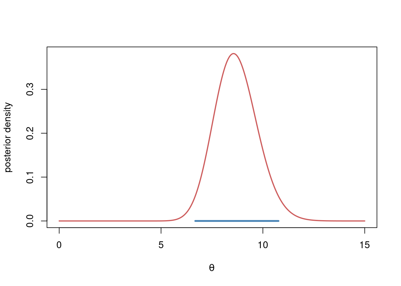
message(paste0("The 95% HPD interval for theta is (", hpd[1], ",", hpd[2],")"))The 95% HPD interval for theta is (6.68168168168168,10.7657657657658)Plot the HPD as a blue line:
plot(thetaGrid, postDens, type = "l", col = "indianred", lwd = 2,
     xlab = expression(theta), ylab = "posterior density")
lines(hpd, c(0,0), col = "steelblue", lwd = 3)