Chapter 3 - Multi-parameter models: Exercise solutions

Author

Mattias Villani

Click on the arrow to see a solution.

Exercise 3.1

A dataset contains observations on measurements of pesticide for \(n=24\) pike fish in a lake in southern Italy. The sample mean pesticide level is \(\bar{x} = 12.5\) with a sample standard deviation of \(s=3.1\). Assume that the pesticide levels \(X_1,\ldots,X_n|\theta,\sigma^2 \sim \mathrm{N}(\theta,\sigma^2)\) are independent and identically distributed normal random variables with unknown mean \(\theta\) and unknown variance \(\sigma^2\).

Compute the joint posterior distribution for \(\theta\) and \(\sigma^2\) using a conjugate prior distribution. Use a prior mean for \(\theta\) of \(8\) and an (imaginary) prior sample size of \(5\). Use \(\sigma_0^2 = 1^2\) and \(\nu_0 = 3\) degrees of freedom in your prior for \(\sigma^2\). Plot the marginal posterior distribution of \(\theta\).

Solution

The posterior distribution is given by \[ \begin{aligned} \theta | \sigma^2 , \boldsymbol{x} &\sim N\Big(\mu_n,\frac{\sigma^2}{\kappa_n}\Big) \\ \sigma^2 | \boldsymbol{x} &\sim \mathrm{Inv-}\chi^2(\nu_n,\sigma_n^2) \end{aligned} \] where \[ \begin{aligned} \mu_n &= w \bar x + (1-w)\mu_0 \\ w &= \frac{n}{\kappa_0+n} \\ \kappa_n &= \kappa_0 + n \\ \nu_n &= \nu_0 + n \\ \nu_n\sigma_n^2 &= \nu_0\sigma_0^2 + (n-1)s^2 + \frac{\kappa_0 n}{\kappa_0+n}(\bar x -\mu_0)^2 \end{aligned} \] We have

# data 
n = 24
xBar = 12.5
s2 = 3.1^2

# prior
mu0 = 8
kappa0 = 5
nu0 = 3
sigma02 = 1^2

# posterior
w = n/(kappa0 + n)
mun = w*xBar + (1-w)*mu0
kappan = kappa0 + n
nun = nu0 + n
sigman2 = (nu0*sigma02 + (n-1)*s2  + 
             (kappa0*n/(kappa0 + n))*(xBar - mu0)^2 )/nun

So the joint posterior is \[ \begin{aligned} \theta | \sigma^2 , \boldsymbol{x} &\sim N\Big(11.724,\frac{\sigma^2}{29}\Big) \\ \sigma^2 | \boldsymbol{x} &\sim \mathrm{Inv-}\chi^2(27,11.401) \end{aligned} \] The marginal posterior for \(\theta\) is \[ \theta \vert \boldsymbol{x} \sim t\Big(\mu_n,\frac{\sigma_n^2}{\kappa_n},\nu_n\Big) = t\Big(27,\frac{11.401}{29},27\Big) \] Plotting the marginal posterior of \(\theta\):

thetaGrid = seq(7, 18, length = 1000)
sigma2Grid = seq(0.001, 30, length = 1000)
dtdist <- function(x, mu, sigma2, nu){
  return((1/sqrt(sigma2))*dt(x = (x - mu)/sqrt(sigma2), df = nu))
}
plot(thetaGrid, dtdist(thetaGrid, mun, sigman2/kappan, nun), type = "l", 
     xlab = expression(theta), ylab = "posterior density", 
     col = "indianred", main = expression(theta))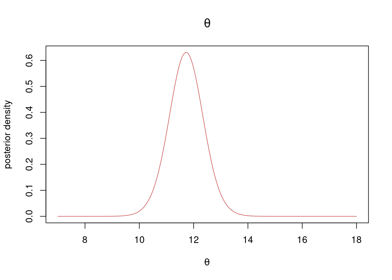

Exercise 3.3

Let \(X_1,\ldots,X_n \mid \theta,\sigma^2 \overset{\mathrm{iid}}{\sim} \mathrm{N}(\theta,\sigma^2)\), where \(\theta\) is assumed known. Show that the \(\mathrm{Inv-}\chi^2\) distribution is a conjugate prior for \(\sigma^2\).

Solution

The normal density function for a single observation \(x_i\) is \[ p(x_i \vert \theta, \sigma^2) = \frac{1}{\sqrt{2\pi\sigma^2}}\exp\Big(-\frac{1}{2\sigma^2}(x_i-\theta)^2\Big) \propto \frac{1}{(\sigma^2)^{1/2}}\exp\Big(-\frac{1}{2\sigma^2}(x_i-\theta)^2\Big) \] The likelihood for the iid normal model with known mean \(\theta\) is therefore the product of \(n\) such density functions: \[ \begin{aligned} p(x_1,\ldots,x_n \vert \theta, \sigma^2) = \prod_{i=1}^n p(x_i \vert \theta, \sigma^2) &\propto \frac{1}{(\sigma^2)^{n/2}}\exp\Big( -\frac{1}{2\sigma^2}\sum_{i=1}^n (x_i-\theta)^2\Big) \\ &\propto \frac{1}{(\sigma^2)^{n/2}}\exp\Big( -\frac{n s^2}{2\sigma^2}\Big) \end{aligned} \] where we have defined \(s^2 = \frac{\sum_{i=1}^n (x_i-\theta)^2}{n}\) as the sample standard deviation (dividing by \(n\) instead of \(n-1\) since the mean \(\theta\) is assumed known).

The density of the \(\sigma^2 \sim \mathrm{Scaled-Inv-}\chi^2(\nu_0,\sigma_0^2)\) prior is of the form \[ p(\sigma^2) \propto \frac{1}{(\sigma^2)^{1+\nu_0/2}}\exp\Big( -\frac{\nu_0\sigma_0^2}{2\sigma^2} \Big) \] The posterior distribution from using the \(\sigma^2 \sim \mathrm{Scaled-Inv-}\chi^2(\nu_0,\sigma_0^2)\) prior is given by Bayes’ theorem as (to avoid cluttering the notation, we do not write out the conditioning on \(\theta\) since it is known) \[ \begin{aligned} p(\sigma^2 \vert x_1,\ldots,x_n) &\propto p(x_1,\ldots,x_n \vert \sigma^2)p(\sigma^2) \\ & \propto \frac{1}{(\sigma^2)^{n/2}}\exp\Big( -\frac{n s^2}{2\sigma^2}\Big) \frac{1}{(\sigma^2)^{1+\nu_0/2}}\exp\Big( -\frac{\nu_0\sigma_0^2}{2\sigma^2} \Big) \\ &\propto \frac{1}{(\sigma^2)^{1+(\nu_0+n)/2}}\exp\Big( -\frac{1}{2\sigma^2}\big( \nu_0 \sigma_0^2 + n s^2 \big) \Big) \\ &= \frac{1}{(\sigma^2)^{1+(\nu_0+n)/2}}\exp\Big( -\frac{\nu_0+n}{2\sigma^2}\frac{\nu_0 \sigma_0^2 + n s^2 }{\nu_0+n} \Big) \end{aligned} \] which is proportional to a \(\sigma^2 \sim \chi^2(\nu_0+n,\frac{\nu_0 \sigma_0^2 + n s^2 }{\nu_0+n})\) density. Note how the location parameter in the posterior \[ \frac{\nu_0 \sigma_0^2 + n s^2 }{\nu_0+n} = \frac{\nu_0}{\nu_0+n} \sigma_0^2 + \frac{n}{\nu_0+n}s^2 \] is a weighted average of prior location \(\sigma_0^2\) and the data estimate \(s^2\), with more weight placed on the strongest information source (prior with \(\nu_0\) imaginary sample data points versus the data with \(n\) actual data points).

Exercise 3.6

A Swedish poll in 2024 asked \(2311\) persons the question: The table below gives the poll results across the eight parties in parliament and the nineth option .

Let \(\boldsymbol{y} = (y_1,\ldots,y_9)\) denote the number of votes for each of the nine parties, where \(y_c\) is the number of votes for party \(c\). Model the data as iid from a multinomial distribution \[\begin{equation*} \boldsymbol{y} \mid \boldsymbol{\theta} \sim \mathrm{Multinomial}(n,\boldsymbol{\theta}), \end{equation*}\] where \(n=2311\) is the total number of respondents and \(\boldsymbol{\theta} = (\theta_1,\ldots,\theta_9)\) is the vector of voting proportions for each party, where \(\theta_c\) is the proportion of votes for party \(c\).

The previous election in 2022 resulted in the following voting percentages:

Use Dirichlet prior \(\boldsymbol{\theta} \sim \mathrm{Dirichlet}(\boldsymbol{\alpha})\) with \(\boldsymbol{\alpha} = (\alpha_1,\ldots,\alpha_9)\). Set the priorhyperparameters based on the election results from 2022, but assuming that the prior information is equivalent to only \(400\) respondents today.

a) What is the posterior distribution for the voting shares?

Solution

Set up data for the current poll, and the results from the election in 2022:

y = c(410, 88, 83, 81, 721, 196, 238, 434, 60)
election2022 = c(19.10, 4.61, 6.71, 5.34, 30.33, 6.75, 5.08, 20.54, 1.54)
proportionElection2022 = election2022/100
alphaPrior = 400*proportionElection2022 # not integers, but that's OK

Compute the posterior hyperparameters by adding up the data count \(y_c\) in each category with its corresponding prior count \(\alpha_c\):

alphaPost = alphaPrior + y

So the (joint) posterior distribution for the Swedish voting shares are \[ \boldsymbol{\theta} \vert \boldsymbol{y} \sim \mathrm{Dirichlet}\Big(486.4, 106.44, 109.84, 102.36, 842.32, 223, 258.32, 516.16, 66.16\Big) \]

b) What is the marginal posterior distribution for the voting share of the S-party? Plot the distribution without resorting to simulation.

Solution

From the properties of the Dirichlet distribution box in the Bayesian Learning book, we know that if \((\theta_1,\ldots,\theta_C) \sim \mathrm{Dirichlet}(\alpha_1,\ldots,\alpha_C)\), then marginal distribution for the probability/proportion in category \(c\) is
\[ \theta_c \sim \mathrm{Beta}(\alpha_c, \alpha_+ -\alpha_c). \] We can apply this result to get the marginal posterior for \(\theta_5\) (the proportion of S-voters), we just need to remember that the parameters in the posterior are \(\alpha_c + y_c\) for \(c=1,\ldots,C\), or alphaPost in the code. The marginal posterior for the proportion of S-party voters is \[ \theta_5 \vert \boldsymbol{y} \sim \mathrm{Beta}\Big(842.32, 1868.68 \Big), \] which we can plot:

thetaGrid = seq(0, 1, length = 1000)
plot(thetaGrid, dbeta(thetaGrid, alphaPost[5], sum(alphaPost) - alphaPost[5]), 
     xlab = "proportion of S-voters", ylab = "posterior density", type = "l", 
     lwd = 3, col = "indianred")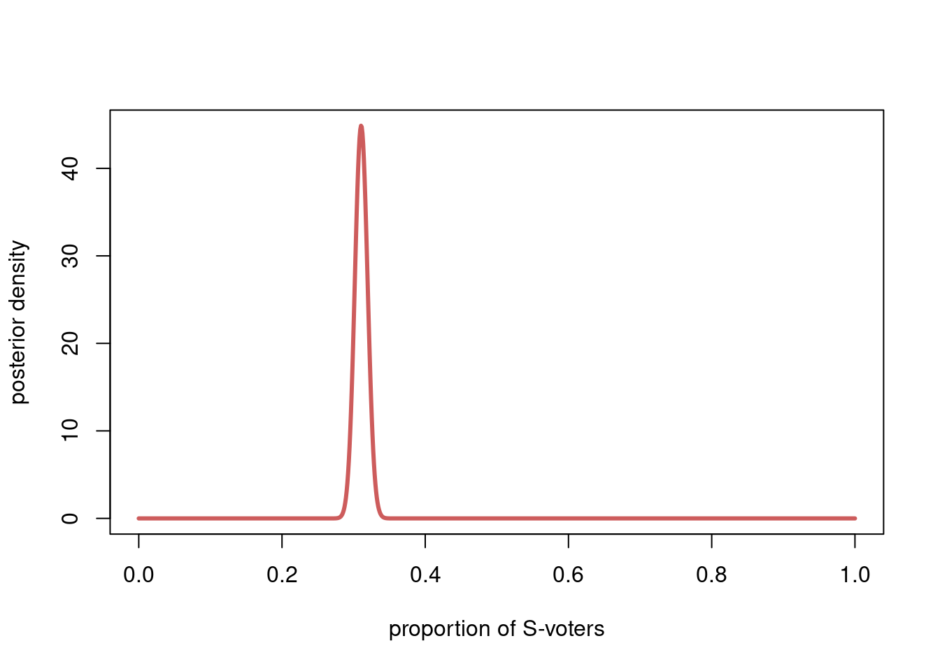

c) A party needs at least 4% of the votes to get into parliament. Use simulation to compute the posterior probability that both L and KD parties do not make it to parliament.

Solution

Define a Dirichlet random number generator using the algorithm in Chapter 3.

rdirichlet <- function(nIter, param){
  nCat <- length(param)
  thetaDraws <- matrix(0,nIter,nCat) #Storage
  for (j in 1:nCat){
    thetaDraws[,j] <- rgamma(nIter, param[j], 1)
  }
  for (i in 1:nIter){
    thetaDraws[i,] = thetaDraws[i,]/sum(thetaDraws[i,])
  }
  return(thetaDraws)
}

Use the simulator to simulate \(10000\) draws from the posterior distribution. For each draw check if both the L and KD party each have less than 4% of the votes.

nSim = 10000
postDraws = rdirichlet(nSim, alphaPost)
bothPartyInParliament = rep(NA, nSim)
for (i in 1:nSim){
  bothPartyInParliament[i] = all(postDraws[i,c(2,4)] < 0.04)
}

The posterior probability that both parties are below \(4\%\) is 0.4318.

Exercise 3.7

The monthly income (in thousands Swedish Krona) of ten randomly selected persons are: 14, 25, 45, 25, 30, 33, 19, 50, 34 and 67. The log-normal distribution (see Box~ and ) is a commonly used model for income distributions. Let \(Y_1,\ldots,Y_n \vert \theta,\sigma^{2}\overset{\mathrm{iid}}{\sim}\mathrm{LN}(\theta,\sigma^{2})\), where \(\theta=\log(33)\) is assumed to be known but \(\sigma^{2}\) is unknown with non-informative prior \(p(\sigma^{2})\propto1/\sigma^{2}\). The posterior for \(\sigma^{2}\) given \(\theta\) is the \(\mathrm{Inv-}\chi^{2}(n,\tau^{2})\) distribution, where \[\begin{equation*} \tau^{2}=\frac{\sum_{i=1}^{n}(\log y_{i}-\theta)^{2}}{n}. \end{equation*}\]

a) Simulate \(10,000\) draws from the posterior of \(\sigma^{2}\), assuming \(\theta=\log(33)\) is known. Plot a histogram of the posterior draws of the \(\sigma\).

Solution

y = c(14, 25, 45, 25, 30, 33, 19, 50, 34, 67)
logy = log(y)
n = length(y)
theta = log(33)
tau2 = sum((logy - theta)^2)/n

# Defining a function that simulates nSim draws
# from the scaled inverse Chi-square distribution
rScaledInvChi2 <- function(nSim, df, scale){
  return((df*scale)/rchisq(nSim, df=df))
}
nSim = 10000
sigma2Draws = rScaledInvChi2(nSim, n, tau2)
hist(sqrt(sigma2Draws), 100, col = "steelblue", main = "", freq = FALSE,
     xlab = expression(sigma), ylab = "posterior density")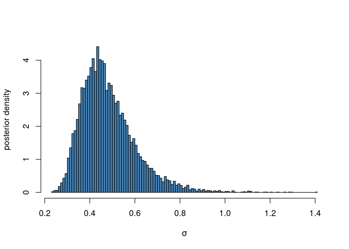

b) A commonly used measure of income inequality is the Gini coefficient, \(0\leq G\leq1\), where \(G=0\) is complete income equality, and \(G=1\) means complete income inequality. It can be shown that \(G=2\Phi\left(\sigma/\sqrt{2}\right)-1\) when incomes follow a \(\mathrm{LN}(\theta,\sigma^{2})\) distribution, where \(\Phi(z)\) is the cumulative distribution function (CDF) for the standard normal distribution. Use the posterior draws from a) to compute the posterior distribution of the Gini coefficient \(G\). Plot a histogram of the posterior draws of \(G\).

Solution

gini = rep(0, nSim)
for (i in 1:nSim){
  gini[i] = 2*pnorm(sqrt(sigma2Draws[i])/sqrt(2)) - 1
} 
hist(gini, 100, col = "cornsilk", main = "", freq = FALSE,
     xlab = "Gini coefficient, G", ylab = "posterior density")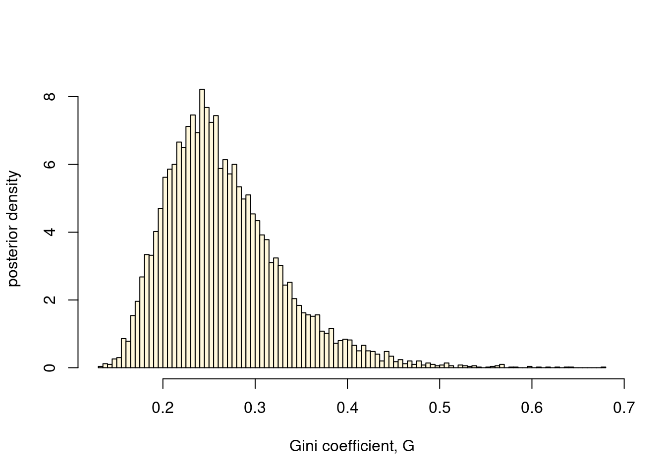

c) Compute a \(95\)% Highest Posterior Density (HPD) interval for \(G\). To compute the HPD interval you will need an estimate of the posterior density for \(G\); a common approach is to use a kernel density estimator, for example the density function in R.

Solution

We first estimate the posterior density from the posterior draws using a kernel density estimator, and plotting it on top of the histogram:

kde = density(gini)
giniGrid = kde$x
postDens = kde$y
hist(gini, 100, col = "cornsilk", main = "", freq = FALSE,
     xlab = "Gini coefficient, G", ylab = "posterior density")
lines(giniGrid, postDens, lwd = 3, col = "indianred")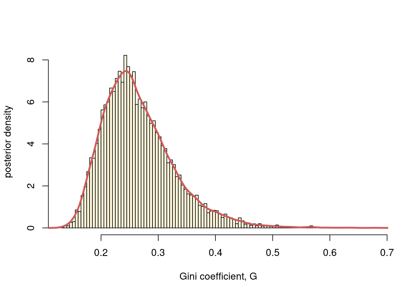

Now that we have the posterior density, and we can see that it is unimodal, we can use the same code as in the Solution to Exercise @q:iid_poisson_ambulance_b.

binWidth = giniGrid[2]- giniGrid[1]
# first, sort the density values from highest to lowest
postDensOrdered = sort(postDens, decreasing = TRUE)  
# reorder the thetaValues so that they still match the density values
giniOrdered = giniGrid[order(postDens, decreasing = TRUE)] 
cumsumPostDens = cumsum(binWidth*postDensOrdered) # posterior cdf 
inHPD = which(cumsumPostDens < 0.95) # find highest pdf vals up to 95% quota.
hpd = c(min(giniOrdered[inHPD]), max(giniOrdered[inHPD]))
message(paste0("The 95% HPD interval for the Gini coefficient is (", hpd[1], ",", hpd[2],")"))

The 95% HPD interval for the Gini coefficient is (0.159044415119536,0.392529484142363)