Chapter 5 - Linear Regression: Exercise solutions

Author

Mattias Villani

Click on the arrow to see a solution.

Exercise 5.1

The BostonHousing data is available in, for example, the mlbench R package. The dataset contains the median house price medv in 506 regions in Boston, {U.S.A.}, as well as data on several characteristics in each of the regions. In this exercise we will model the log of the median house price as a function of a subset of the covariates: logmedv where logmedv is the log of medv, crim is the per capita crime rate by town, age is the proportion of owner-occupied units built prior to 1940, and ptratio is the pupil-teacher ratio by town. Use the conjugate prior \[\begin{align*} \beta_j \vert \sigma^2 & \sim N(\boldsymbol{0},10^2\sigma^2 \boldsymbol{I}_p)\\ \sigma^2 & \sim \mathrm{Inv}-\chi^2(3,0.5^2). \end{align*}\] where \(\boldsymbol{I}_p\) is a \(p \times p\) identity matrix and \(p=4\) is the number of regression coefficients including the intercept.

Compute the marginal posterior distribution for each \(\beta_j, j=1,\ldots,4\) and plot each marginal density. Do not use simulation methods, but a computer is advisable for the matrix operations. Compute the posterior mean and a 95% equal-tail credible interval for each \(\beta_j\). Use the credible intervals to test the four separate hypotheses that \(\beta_j = 0\) for \(j=1,\ldots,4\). Which of the covariates are important in the model?

\(\textit{Hint}\): The general student-\(t\) is not always available in all programming languages (for example in R and Julia), only the standard student-\(t\) \(t(0,1,\nu)\) with location \(0\) and scale \(1\). However, if \(X \sim t(\mu,\sigma^2,\nu)\), then \(Z = (X-\mu)/\sigma \sim t(0,1,\nu)\), so you can use this transformation to compute the density and quantiles of the general student-\(t\) distribution. This means that the density of \(X\) can be computed as \[\begin{equation*} p(x) = \frac{1}{\sigma} p\Big(\frac{x-\mu}{\sigma}, \nu \Big), \end{equation*}\] where \(p(z, \nu)\) is the density of the standard student-\(t\) distribution with \(\nu\) degrees of freedom. Similarly, the \(\alpha\) quantile of \(X\) can be computed as \[\begin{equation*} x_\alpha = \mu + \sigma t_\alpha, \end{equation*}\] where \(t_\alpha\) is the \(\alpha\) quantile of the standard student-\(t\) distribution.

Solution

First, we set up the data by loading it and setting up the response vector and matrix of covariates:

library(mlbench)
data("BostonHousing", package = "mlbench")
y = log(BostonHousing$medv)
X = cbind(1, BostonHousing$crim, BostonHousing$age, BostonHousing$ptratio)
n = dim(X)[1]
p = dim(X)[2]

Next we set up the prior

mu0 = rep(0, p)
Omega0 = 10^(-2)*diag(p)
nu0 = 3
sigma20 = 0.5^2

From Chapter 5 in the book, the joint posterior distribution of all \(\beta\) coefficients is given by a multivariate-\(t\) distribution \[ \boldsymbol{\beta} \vert \boldsymbol{y} \sim t\big(\boldsymbol{\mu}_n, \sigma_n^2\boldsymbol{\Omega}_n^{-1}, \nu_n \big) \] where

\(\boldsymbol{\Omega}_n = \boldsymbol{X}^\top\boldsymbol{X} + \boldsymbol{\Omega}_0\)
\(\boldsymbol{\mu}_n = \boldsymbol{\Omega}_n^{-1}(\boldsymbol{X}^\top\boldsymbol{X}\hat{\boldsymbol{\beta}} + \boldsymbol{\Omega}_0\boldsymbol{\mu}_0)\)
\(\hat{\boldsymbol{\beta}} = (\boldsymbol{X}^\top\boldsymbol{X})^{-1}\boldsymbol{X}^\top \mathbf{y}\)
\({\nu}_n = \nu_0 + n\)
\(\sigma^2_n = \Big( \nu_0\sigma_0^2 + (n-p)s^2 + (\boldsymbol{\mu}_n -\hat{\boldsymbol{\beta}})^\top \boldsymbol{X}^\top\boldsymbol{X}(\boldsymbol{\mu}_n -\hat{\boldsymbol{\beta}}) + (\boldsymbol{\mu}_n - \boldsymbol{\mu}_0)^\top \boldsymbol{\Omega}_0(\boldsymbol{\mu}_n - \boldsymbol{\mu}_0 ) \Big) / \nu_n\)

The marginal posterior distribution for each \(\beta_j\) is a univariate student-\(t\) distribution \[ \beta_j \sim t(\mu_{n,j}, \sigma^2_{\beta,j}, \nu_n) \] where \(\mu_{n,j}\) is the \(j\)th element of \(\boldsymbol{\mu}_n\) and \(\sigma^2_{\beta,j}\) is the \(j\)th diagonal element of \(\sigma_n^2\boldsymbol{\Omega}_n^{-1}\).

We start by computing the hyperparameters of the joint posterior of \(\boldsymbol{\beta}\):

betaHat = solve(t(X)%*%X) %*% (t(X) %*% y) 
Omegan = t(X)%*%X + Omega0
mun = solve(Omegan) %*% (t(X)%*%X %*% betaHat + Omega0 %*% mu0)
nun = nu0 + n
sigma2n = as.numeric((nu0*sigma20 + ( t(y)%*%y + t(mu0)%*%Omega0%*%mu0 - t(mun)%*%Omegan%*%mun))/nun)

Now we can just extract the relevant element for each marginal posterior of \(\beta_j\) and plot each univariate student-\(t\) density:

# Defining a general student-t distribution with three parameters
dtgeneral <- function(x, mu, sigma2, nu){
  t = (x - mu)/sqrt(sigma2) # standardized variable
  dens = dt(t, nu)/sqrt(sigma2)
  return(dens)
}

# quantile function general student-t
qtgeneral <- function(prob, mu, sigma2, nu){
  return(mu + sqrt(sigma2)*qt(prob, nu))
}

covMarginalPost = sigma2n*solve(Omegan)
stdMarginalPost = sqrt(diag(covMarginalPost))
par(mfrow = c(2,2))
CI = matrix(rep(2*p), p, 2)
for (j in 1:p){
  betaGrid = seq(mun[j] - 4*stdMarginalPost[j], mun[j] + 4*stdMarginalPost[j], length = 1000)
  margDens = dtgeneral(betaGrid, mun[j], covMarginalPost[j,j], nun)
  plot(betaGrid, margDens, type = "l", col = "cornflowerblue")
  CI[j,1] = qtgeneral(0.025, mun[j], covMarginalPost[j,j], nun)
  CI[j,2] = qtgeneral(0.975, mun[j], covMarginalPost[j,j], nun)
  message(paste("The 95% CI for beta", j, " is (", round(CI[j,1],3), " , ", round(CI[j,2],3), ")"))
}

The 95% CI for beta 1  is ( 4.273  ,  4.742 )

The 95% CI for beta 2  is ( -0.02  ,  -0.013 )

The 95% CI for beta 3  is ( -0.005  ,  -0.003 )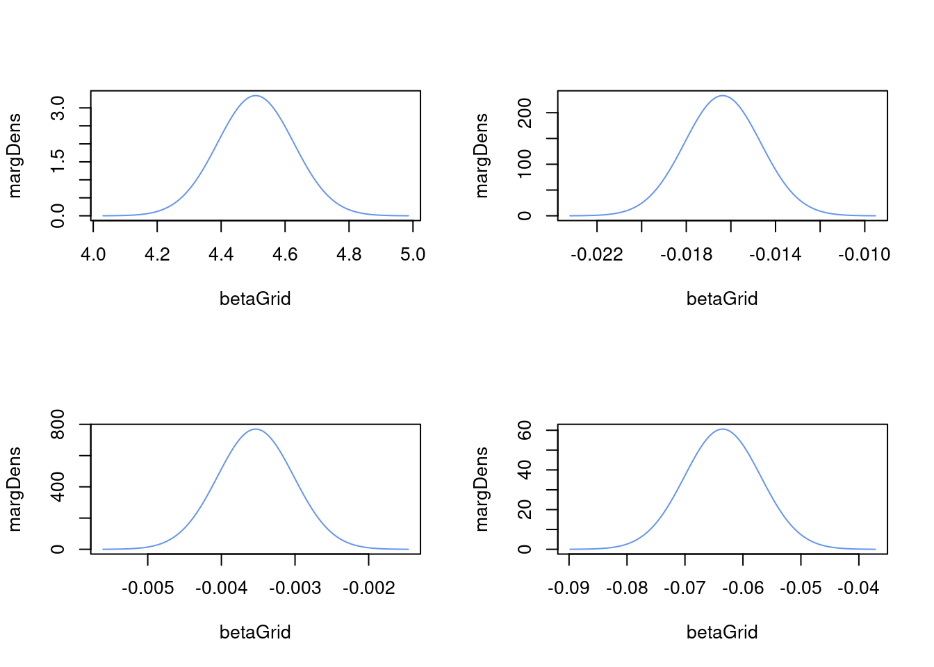

The 95% CI for beta 4  is ( -0.076  ,  -0.051 )

The value \(\beta_j=0\) is not included in any of the 95% credible intervals. The value \(\beta_j=0\) is therefore not probable given the data, so we can reject the null hypothesis of no effect for all covariates. Note that this is not a frequentist test, but rather a Bayesian version of such a test. There are other ways to do Bayesian hypothesis testing using Bayes factor and Bayesian variable selection, but the credible interval approach has the advantage of being robust to the choice of prior.