Chapter 6 - Prediction and Decision making: Exercise solutions

Click on the arrow to see a solution.

Exercise 6.1

Let \(X_{1},\ldots,X_{n}\overset{iid}{\sim}\mathrm{Bern}(\theta)\), with a \(\mathrm{Beta}(\alpha,\beta)\) prior for \(\theta\).

a) Derive the predictive distribution for \(X_{n+1}\) conditional on having observed \(x_1,\ldots,x_n\).

Solution TBD

b) You need to decide if you bring your umbrella during your daily walk. It has rained on two days during the last ten days, and you assess those ten days to be representative of the weather today, the 11th day. Your utility for the action-state combinations are given in the table below. Assume a \(\theta \sim \mathrm{Beta}(1,1)\) prior. Compute the Bayesian decision.

Solution TBD

c) How sensitive is your decision in b) to the changes in the prior hyperparameters, \(\alpha\) and \(\beta\)?

Solution TBD

---

Exercise 6.2

Let \(X_1,\ldots,X_n \vert \theta \overset{\mathrm{iid}}{\sim} \mathrm{Expon}(\theta)\), and assume the conjugate \(\mathrm{Gamma}(\alpha,\beta)\) prior for \(\theta\).

a) Derive the predictive distribution for a new observation \(\tilde{X}_{n+1}\) conditional on having observed \(x_1,\ldots,x_n\).

Solution

The predictive distribution for the next observation \(\tilde{X}_{n+1}\) is \[ p(\tilde{x}_{n+1} \vert x_1,\ldots,x_n) = \int p(\tilde{x}_{n+1} \vert \theta) p(\theta \vert x_1,\ldots,x_n) d\theta \] where \(\theta \vert x_1,\ldots,x_n \sim \mathrm{Gamma}(\alpha + n, \beta + \sum_{i=1}^n x_i)\) and \(p(\tilde{x}_{n+1} \vert \theta)\) is the pdf of the exponential distribution. So, \[ \begin{aligned} p(\tilde{x}_{n+1} \vert x_1,\ldots,x_n) &= \int \theta e^{-\theta\tilde{x}_{n+1}}\cdot\frac{\left(\beta+n\bar{x}\right)^{\alpha+n}}{\Gamma(\alpha+n)}\theta^{\alpha+n-1}e^{-(\beta+n\bar{x})\theta}d\theta \\ &= \frac{\left(\beta+n\bar{x}\right)^{\alpha+n}}{\Gamma(\alpha+n)}\int \theta^{(\alpha+n + 1) -1}e^{-(\beta+n\bar{x} + \tilde{x}_{n+1})\theta}d\theta \\ \end{aligned} \] The integral \(\int \theta^{(\alpha+n + 1) -1}e^{-(\beta+n\bar{x} + \tilde{x}_{n+1})\theta}d\theta\) is the integral of the unnormalized density function of the \(\mathrm{Gamma}(\alpha+n + 1, \beta+n\bar{x} + \tilde{x}_{n+1})\) distribution. Hence the integral can be directly obtained from the normalizing constant of this distribution and we obtain \[ p(\tilde{x}_{n+1} \vert x_1,\ldots,x_n) = \frac{\left(\beta+n\bar{x}\right)^{\alpha+n}}{\Gamma(\alpha+n)}\frac{\Gamma(\alpha+n+1)}{(\beta+n\bar{x} + \tilde{x}_{n+1})^{\alpha+n+1}} \] This density is not among the really famous ones, but it has a name, the Compound Gamma distribution; see the Compound Gamma distribution widget, if you are curious. The distribution in the widget is actually a little more general, but set the hyperparameter \(\kappa=1\) to get the distribution here. Hence, using the notation in the widget, the predictive distribution is \[ \tilde{X}_{n+1} \sim \mathrm{CompoundGamma}(\alpha+n, \beta + n\bar{x}, 1) \] Note that the density expression above is a little messy mainly because of the normalizing constant. We can remove normalization constants and write \[ p(\tilde{x}_{n+1} \vert x_1,\ldots,x_n) \propto \frac{1}{(\beta+n\bar{x} + \tilde{x}_{n+1})^{\alpha+n+1}} \] where it is important to rememeber that we are here interested in the distribution of \(\tilde{x}_{n+1}\), so all terms involving \(\tilde{x}_{n+1}\) must be kept.

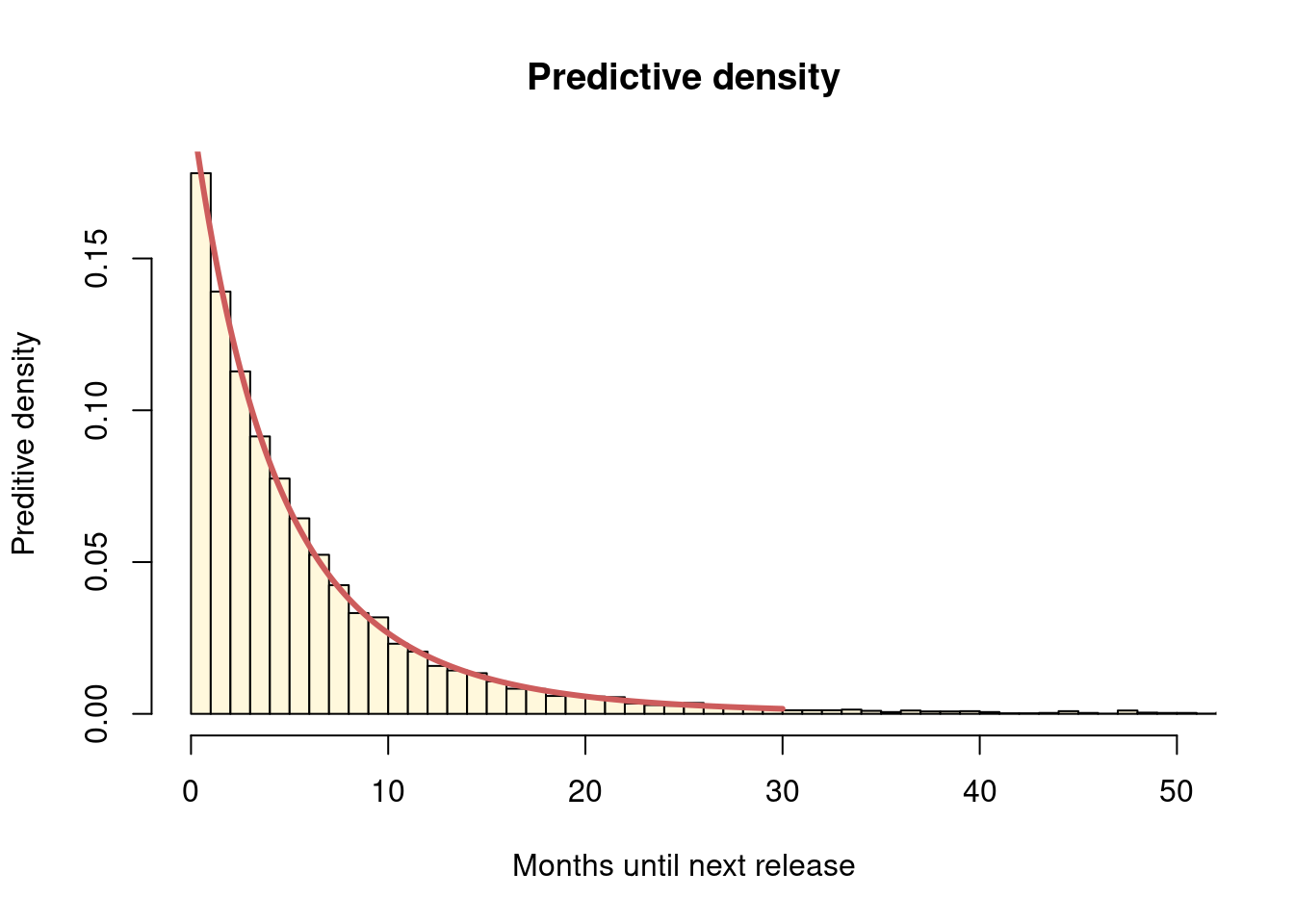
b) A medium size software project is interested in predicting the time until the next release. The five most recent releases took: \(1.58, 7.02, 8.28, 4.67\) and \(4.05\) months to complete. Previous experience from many simular projects suggests that these completion times can be modelled by an exponential distribution with parameter \(\theta\). The project leader believes that the average completion time is around 3 months, but she is not very certain about this, so you decide to use a \(\mathrm{Gamma}(1/3,1)\) prior for \(\theta\) (recall that the mean of \(\mathrm{Expon}(\theta)\) is \(1/\theta\) not \(\theta\)).

Use simulation to compute the predictive distribution for the time until the next release given the observed data, and plot a histogram. Overlay a density curve using the result in a). The company could go bankrupt if the next release takes more than 18 months to complete Use the draws from the predictive distribution to compute the probability of this catastrophic event.

Solution

The following code plots the predictive density using both simulation and with the analytical result from a).

The simulation from the predictive distribution is performed by :

• first simulating \(m\) draws from the posterior of the parameter \(\theta \vert x_1,\ldots,x_5 \sim \mathrm{Gamma}(\alpha+n, \beta + n\bar{x})\), and then
• for each parameter draw \(\theta^{(i)}\) simulating predictive draws \(\tilde{X}_6^{(i)}\) from the exponential model \(\tilde{X}_6^{(i)} \vert x_1,\ldots,x_5 \sim \mathrm{Expon}(\theta^{(i)})\) for \(i=1,\ldots,m\).

# Set up data and compute posterior hyperparameters
x = c(1.58, 7.02, 8.28, 4.67, 4.05)
n = length(x)
xbar = mean(x)
alphaPrior = 1/3
betaPrior = 1
alphaPost = alphaPrior + n
betaPost = betaPrior + n*xbar

# Simulate from predictive distribution and plot histogram
nSim = 10000
thetaDraws = rgamma(nSim, alphaPost, betaPost)
xPredDraws = rexp(nSim, thetaDraws)
hist(xPredDraws, 100, col = "cornsilk", freq = FALSE,  xlim = c(0,50),
     main = "Predictive density", 
     xlab = "Months until next release", ylab = "Preditive density")

# Defining the general Compound-Gamma density even though we have kappa = 1
dCompoundGamma <- function(x, alpha, beta_, kappa){
  dens = (beta_^alpha/gamma(alpha)) * 
    (gamma(alpha + kappa)/gamma(kappa)) * 
    x^(kappa-1)/(beta_ + x)^(alpha + kappa)
  return(dens)
}

# Overlaying the analytical density for the Compound Gamma distribution
xPredGrid = seq(0, 30, length = 1000)
lines(xPredGrid, dCompoundGamma(xPredGrid, alphaPost, betaPost, 1), 
      lwd = 3, col = "indianred")

The predictive probability that the release takes more than 18 months is not very likely, but cannot be completely ruled out:

mean(xPredDraws > 18)

[1] 0.0626

---

Exercise 6.3

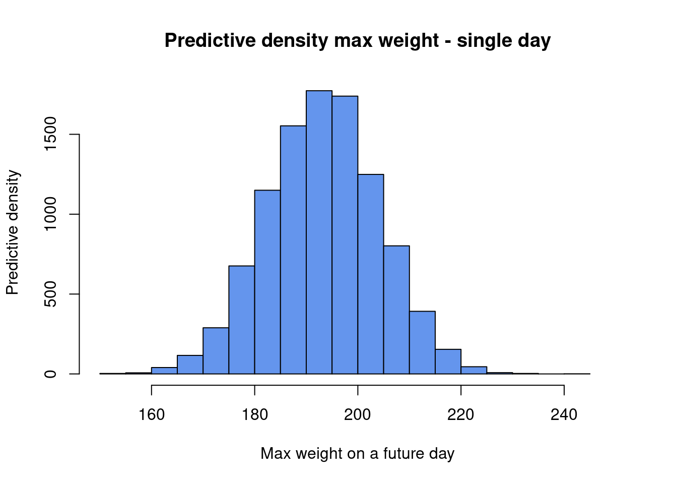
A city considers building a new road bridge for a total cost of \(a\) dollars. The weight that the bridge can hold (\(y\)) at any given time is related to the build cost (\(a\)) as follows \[ y = 10a \] The city has collected data on the maximal weight on the road during five different days: \(y_{1}=190,y_{2}=193,y_{3}=192,y_{4}=197\) and \(y_{5}=188\). Assume the model \(Y_{1},...,Y_{5}\vert\theta \sim N(\theta,\sigma^{2})\), where \(\sigma^{2}\) is assumed known at \(\sigma^{2}=10^{2}\). Assume a \(N(200,10^2)\) prior for \(\theta\).

a) Simulate from the predictive distribution of the maximal weight on . Plot a histogram of the simulated values.

Solution

The predictive distribution for the maximal weight on a future day is \[ \tilde{X} \sim N(\mu_n, \sigma^2 + \tau_n^2), \] where \(\mu_n\) and \(\tau_n^2\) are computed using the formula for the posterior in the iid normal model with known variance in Chapter 2:

y = c(190,193, 192, 197, 188)
n = length(y)
yBar = mean(y)
sigma = 10
mu0 = 200
tau0 = 10
w = (n/sigma^2)/(n/sigma^2 + 1/tau0^2)
mun = w*yBar + (1-w)*mu0
taun2 = 1/( n/sigma^2 +  1/tau0^2 )
predDraws = rnorm(10000, mun, sqrt(sigma^2 + taun2))
hist(predDraws, xlim = c(150,250),
     xlab = "Max weight on a future day", ylab = "Predictive density", 
     main = "Predictive density max weight - single day", col = "cornflowerblue")

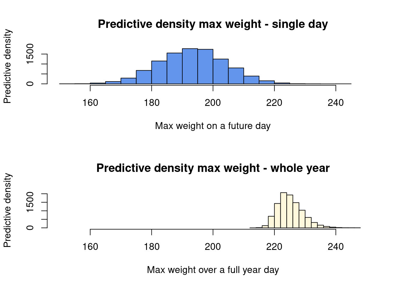
b) Simulate from the predictive distribution of the maximal weight \(\tilde{Y}\) over . Plot a histogram of the simulated values.

Solution

To obtain the predictive distribution for the maximal weight over a whole year we just simulate max weight for \(365\) independent days and take the maximum over all days.

nSim = 10000
maxWeightYear = rep(0, nSim)
for (i in 1:nSim){
  maxWeightYear[i] = max(rnorm(365, mun, sqrt(sigma^2 + taun2)))
}
par(mfrow = c(2,1))
hist(predDraws, xlim = c(150,250),
     xlab = "Max weight on a future day", ylab = "Predictive density", 
     main = "Predictive density max weight - single day", col = "cornflowerblue")
hist(maxWeightYear, , xlim = c(150,250), xlab = "Max weight over a full year day", 
     ylab = "Predictive density", 
     main = "Predictive density max weight - whole year", col = "cornsilk")

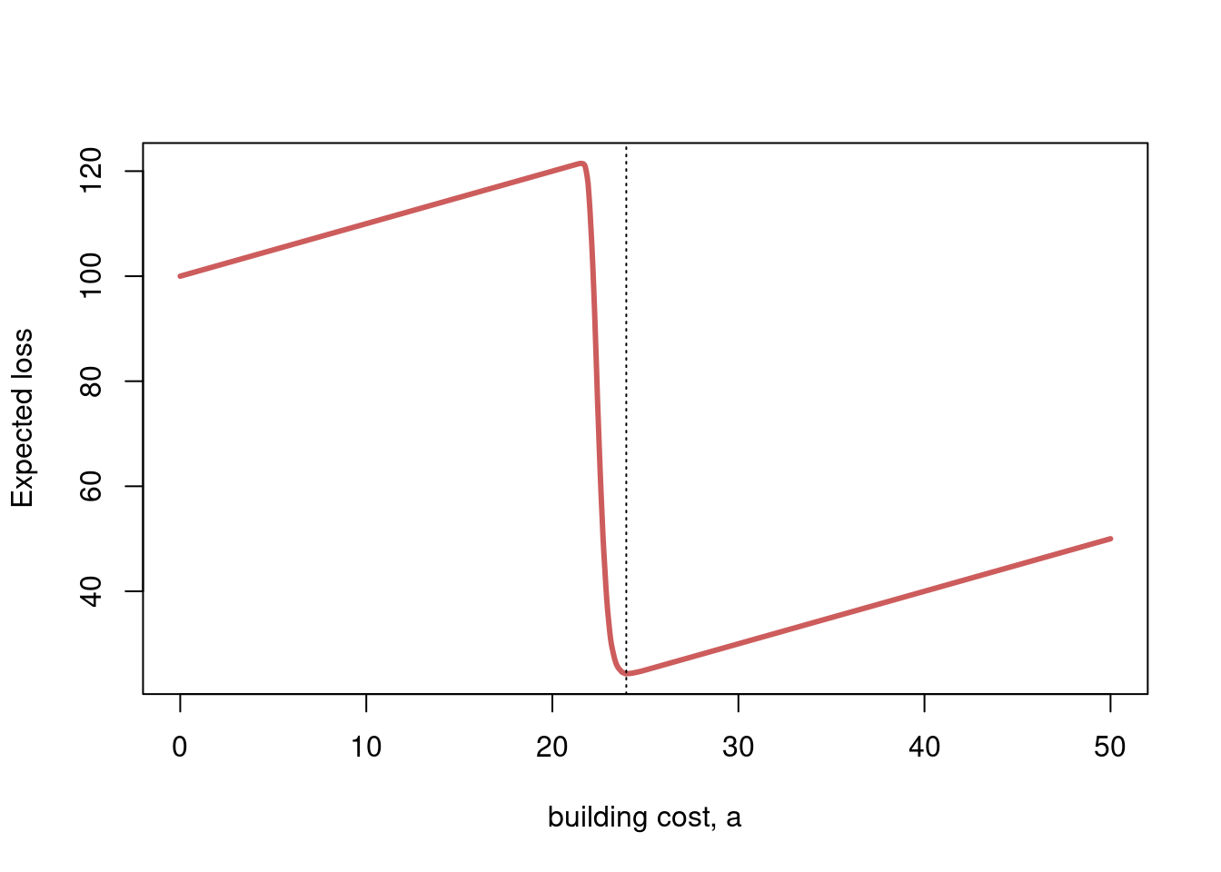
c) The loss function for the building project is \[ L(a, \tilde{Y}) = \begin{cases} a & \text{if } \tilde{Y} \leq 10a \,\,\text{ (bridge holds up)}\\ a + 100 & \text{if } \tilde{Y} > 10a \,\,\text{ (bridge collapses)} \end{cases} \] where \(\tilde{Y}\) is the maximal weight on the bridge during the first year. Hence, we assume that there is no loss after the first year, regardless of what happens. Determine the optimal build cost (\(a\)) using a Bayesian approach.

Solution

We choose the action (building cost \(a\), hence the action space is all \(a>0\)) that minimizes the expected loss, \(EL(a) = \mathbb{E}(L(a,\tilde{Y}))\). The only uncertain factor is maximal weight in the coming year: \(\tilde{Y}\). \[ \begin{aligned} EL(a) = E\left[L(c,\tilde{Y} )\right] & = a\cdot\mathrm{Pr}(\text{bridge holds}\vert a,y_{1},...,y_{5})+(100+a)\cdot\mathrm{Pr}(\text{bridge collapses}\vert a,y_{1},...,y_{5}) \\ & = a\cdot\mathrm{Pr}(\tilde{Y} \leq 10a \vert a,y_{1},...,y_{5})+(100+a)\cdot\mathrm{Pr}(\tilde{Y} > 10a \vert a,y_{1},...,y_{5}) \end{aligned} \] We can compute the expected loss for a range of actions \(a\) using the simulated draws of the maximal weight during the coming year, \(\tilde{Y}\), from b). The expected loss (EL) is plotted as function of \(a\) below.

aGrid = seq(0, 50, length = 1000)
EL = rep(length(aGrid))
for (i in 1:length(aGrid)){
  a = aGrid[i]
  EL[i] = a*mean(maxWeightYear <= 10*a) + (100+a)*mean(maxWeightYear > 10*a)
}
plot(aGrid, EL, xlab = "building cost, a", ylab = "Expected loss", type = "l", 
     lwd = 3, col = "indianred")
abline(v = aGrid[which.min(EL)], lty = "dotted")

The optimal building cost 23.974 is marked out by a dotted vertical line.

---