Chapter 7 - Normal approximation: Exercise solutions

Author

Mattias Villani

Click on the arrow to see a solution.

Exercise 7.1

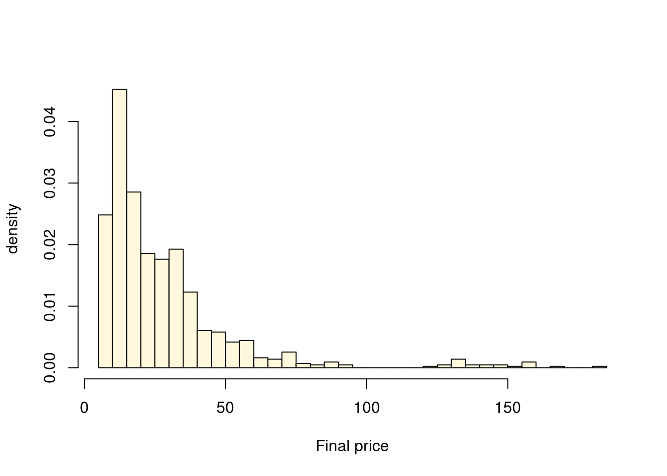
The dataset ebay.csv available at contains the final selling price (FinalPrice) in \(1000\) eBay auctions for collectors coins. We will here only consider the final price of the sold coins, and we discard the auctions with unsold coins (FinalPrice=NA) and the single auction with FinalPrice\(=0\). We model the final price \(Y_i\) in auction \(i\) using a Gamma distribution \[\begin{equation*} Y_i \vert \alpha,\beta \sim \mathrm{Gamma}(\alpha,\beta), \end{equation*}\] where \(\alpha>0\) is the shape parameter and \(\beta>0\) is the rate parameter. Our aim is the posterior distribution \(p(\alpha, \beta \vert \mathbf{y})\) conditional on the data \(\mathbf{y}\), the selling prices in the auctions with at least one bidder. Since both parameters are strictly positive we re-parameterize the model using the exponential function \[\begin{align*} \alpha &= \exp(\theta_1)\\ \beta &= \exp(\theta_2). \end{align*}\] where both \(\theta_1\) and \(\theta_2\) are free to take on any value in \((-\infty,\infty)\). Use the prior \[\begin{align*} \theta_1 &\sim N(0, \tau^2)\\ \theta_2 &\sim N(0, \tau^2) \end{align*}\] and we set \(\tau=10\) to get a weakly informative prior.

We start off by loading the data:

data = read.csv("https://raw.githubusercontent.com/mattiasvillani/BayesianLearningBook/main/data/ebaybids.csv")
y = data$FinalPrice[!is.na(data$FinalPrice) & (data$FinalPrice>0)]
hist(y, 30, freq = FALSE, col ="cornsilk", 
     xlab = "Final price", ylab = "density", main = "")

a) Determine a normal approximation of the posterior distribution \(p(\boldsymbol{\theta} | \mathbf{y})\) based on numerical optimization, where \(\boldsymbol{\theta} = (\theta_1,\theta_2)^\top\).

Solution

We use the normal approximation suggested by the Bernstein-von Mises theorem: \[ \boldsymbol{\theta} \overset{\mathrm{approx}}{\sim} N(\tilde{\boldsymbol{\theta}}, \boldsymbol{J}^{-1}_{\mathbf{y}}) \] where the posterior mode \(\tilde{\boldsymbol{\theta}}\) and posterior information matrix \(\boldsymbol{J}^{-1}_{\mathbf{y}}\) are obtained by numerical optimization. To use optim in R we need to code up the log posterior function

logPostGamma <- function(theta, y, tau){
  alpha = exp(theta[1])
  beta_ = exp(theta[2])
  logLik = sum(dgamma(y, alpha, beta_, log = TRUE))
  logPrior = dnorm(0, tau, log = TRUE) + dnorm(0, tau, log = TRUE)
  return(logLik + logPrior)
}

We can then find all the quantities needed for the normal approximation by running optim.

tau = 10
initVal <- c(0,0) # these initial values imply a Gamma(1,1) distribution.
OptimResults<-optim(initVal, logPostGamma, gr=NULL, y[1:260], tau,
  method = c("BFGS"), control = list(fnscale=-1), hessian=TRUE)
postMode = OptimResults$par
postCov = -solve(OptimResults$hessian)

The normal posterior approximation thus has mean vector

postMode

[1]  0.695345 -2.577673

and covariance matrix

postCov

           [,1]        [,2]
[1,] 0.00663615 0.006636150
[2,] 0.00663615 0.008555005

from which we can compute the approximate posterior standard deviations:

postStd = sqrt(diag(postCov))

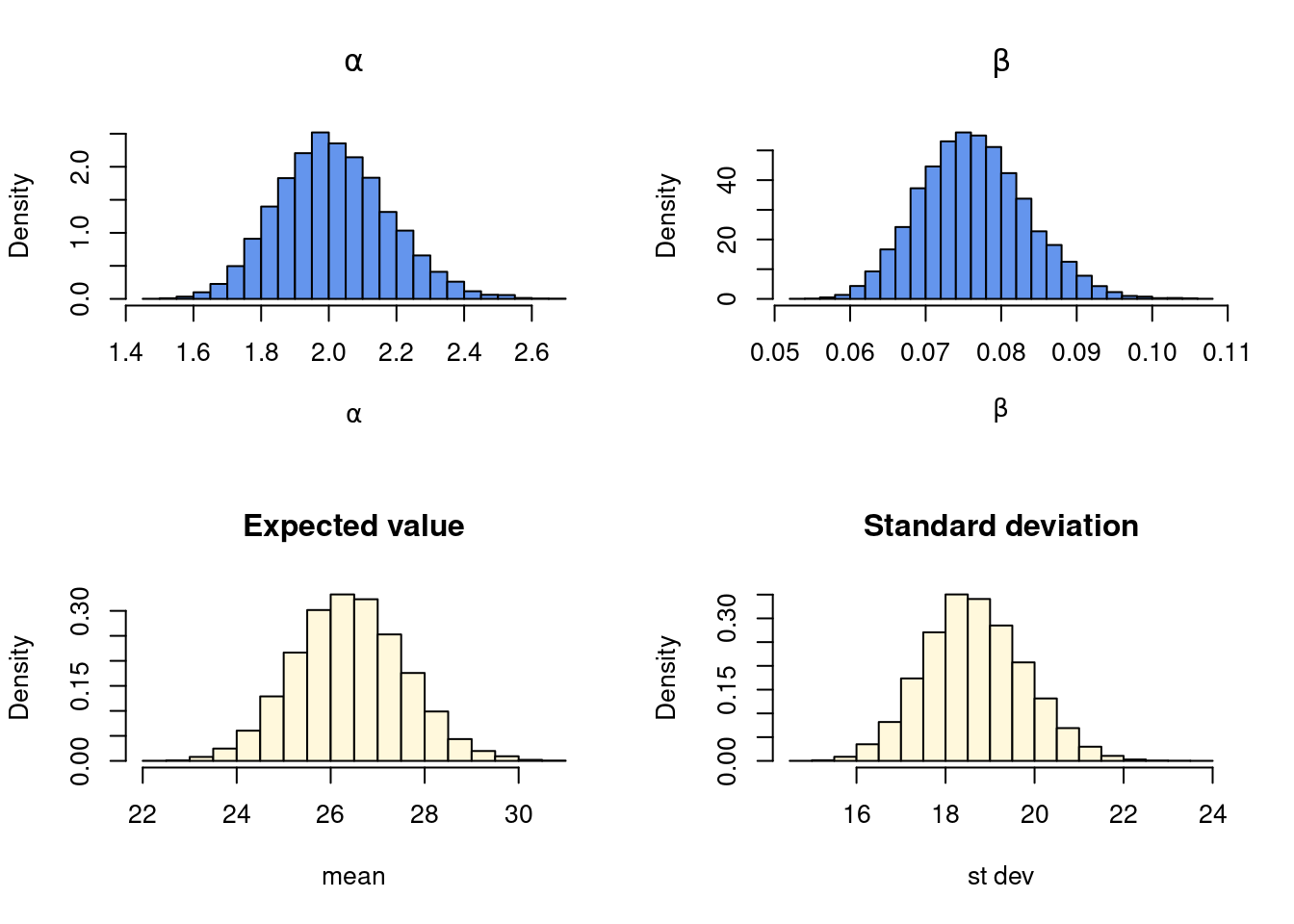
b) Combine the approximation from a) and simulation to approximate the marginal posterior for the original parameters \(\alpha\) and \(\beta\), as well as the marginal posterior of the mean \(\alpha/\beta\) and standard deviation \(\sqrt{\alpha}/\beta\) of the fitted Gamma distribution.

Solution

We use the mvtnorm package to simulate from the normal approximation and then compute the transformation for each draw for \(j=1,\ldots,m\): \[ \begin{aligned} \alpha^{(i)} &= \exp\big(\theta_1^{(i)} \big) \\ \beta^{(i)} &= \exp\big(\theta_2^{(i)} \big) \end{aligned} \] We can then further compute the mean \(\alpha/\beta\) and standard deviation \(\sqrt{\alpha}/\beta\) for each draw. Here is the code:

library(mvtnorm)
nSim = 10000
thetaDraws = rmvnorm(nSim, postMode, postCov)
alphaDraws = exp(thetaDraws[,1])
betaDraws = exp(thetaDraws[,2])
meanDraws = alphaDraws/betaDraws
stdDraws = sqrt(alphaDraws) / betaDraws
par(mfrow = c(2,2))
hist(alphaDraws, 30, freq = FALSE, main = expression(alpha), 
     xlab = expression(alpha), col = "cornflowerblue")
hist(betaDraws, 30, freq = FALSE, main = expression(beta), 
     xlab = expression(beta), col = "cornflowerblue")
hist(meanDraws, 30, freq = FALSE, main = "Expected value", xlab = "mean", 
     col = "cornsilk")
hist(stdDraws, 30, freq = FALSE, main = "Standard deviation", 
     xlab = "st dev", col = "cornsilk")