Bayesian nonlinear regression in RStan

Polynomial regression with L2-regularization prior

Model

This notebook illustrate how to do a Bayesian analysis using rstan for the polynomial regression model $$y={\beta }_0+{\beta }_{1}x+{\beta }_2{x}^2+\dots +{\beta }_p{x}^p+\epsilon ,\epsilon \stackrel{\mathrm{iid}}{\sim }N(0,{\sigma }^2).$$

Prior

An L2-prior (ridge) is used to prevent overfitting $${\beta }_j|{\sigma }^2\stackrel{\mathrm{iid}}{\sim }N(0,\frac{{\sigma }^2}{{\lambda }^2}),$$ where the regularization parameter $\lambda$ is learned from the data. The regularization parameter $\lambda$ is a precision (inverse variance) and we will here instead parameterize it as a variance: ${\psi }^2=1/\lambda$ in the sampling and use the prior $${\psi }^2\sim \mathrm{Inv}-{\chi }^2({\omega }_0,{\psi }_0^2).$$ The intercept is not regularized and is given a separate prior $${\beta }_0\sim N(0,{\sigma }_{0,\mathrm{intercept}}^2)$$ The noise variance is assign the usual scaled inverse chi-squared prior $${\sigma }^2\sim \mathrm{Inv}-{\chi }^2({\nu }_0,{\sigma }_0^2).$$

Rstan: Install, load, use all cores and no recompile unless needed

#install.packages("rstan", repos = c('https://stan-dev.r-universe.dev', 
#                                    getOption("repos")))
suppressMessages(library(rstan))
options(mc.cores = parallel::detectCores())
rstan_options(auto_write = TRUE)

Load the fossil data ¹

# Read and transform data
rawdata <- read.csv(
  file = "https://github.com/mattiasvillani/introbayes/raw/main/data/fossil.csv"
)
n  = dim(rawdata)[1]
y = rawdata$strontium_ratio
x = rawdata$age
plot(x, y, pch = 16, ylab = "strontium_ratio", xlab = "age", col = colors[1], 
     main = "fossil data")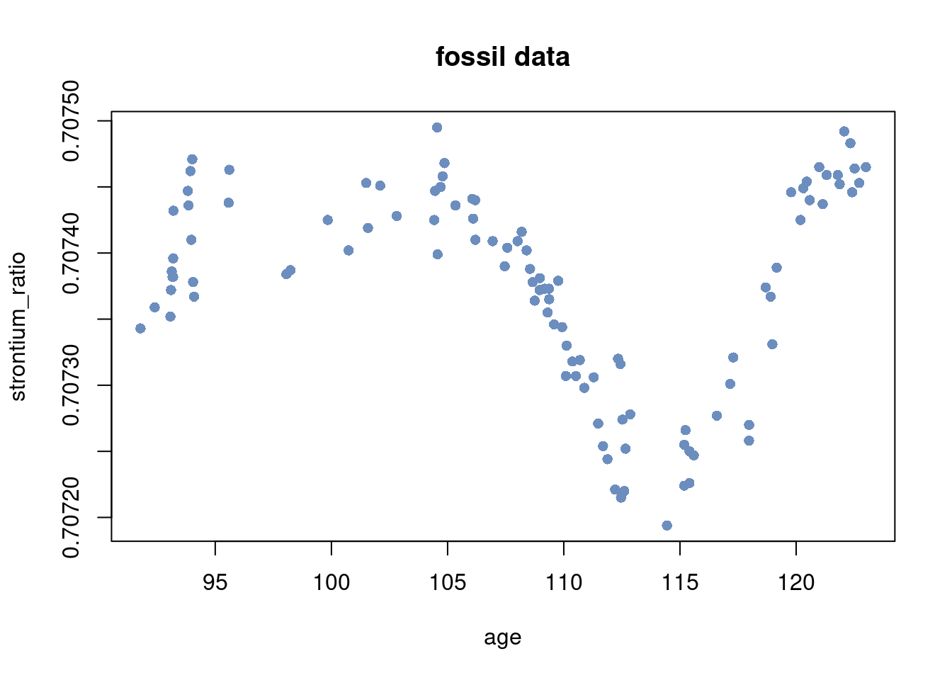

Standardize the covariates and the response variable

mean_y = mean(y)
mean_x = mean(x)
sd_y = sd(y)
sd_x = sd(x)
y = (y - mean_y)/sd_y
x = (x - mean_x)/sd_x

Set up covariate matrix from 10 degree polynomial

degree = 10 # polynomial degree
X = matrix(rep(0, n*degree), n, degree)
for (k in 1:degree){
  X[, k] = x^k
}
p = dim(X)[2]

Setup stan data structures and set prior hyperparameters values

data <- list(n = length(y), p = p, X = X, y = y)
prior <- list(sigma0_intercept = 100, nu0 = 2, sigma20 = 0.11, omega0 = 10, 
              psi20 = 100)

Set up stan model (can also be defined in a separate file)

l2regression = '
data {
  // data
  int<lower=0> n;   // number of observations
  int<lower=0> p;   // number of covariates
  matrix[n, p] X;   // covariate matrix
  vector[n] y;      // response vector
  // prior
  real<lower=0> sigma0_intercept;
  real<lower=0> nu0;
  real<lower=0> sigma20;
  real<lower=0> omega0;
  real<lower=0> psi20;
}
parameters {
  real beta0;            // intercept
  vector[p] beta;        // regression coefficients
  real<lower=0> sigma2;  // error standard deviation
  real<lower=0> psi2;    // psi2 = 1 / lambda, in the usual L2-regularization 
}
model {
  beta0 ~ normal(0, sigma0_intercept);
  sigma2 ~ scaled_inv_chi_square(nu0, sqrt(sigma20));
  psi2 ~ scaled_inv_chi_square(omega0, sqrt(psi20));
  beta ~ normal(0, sqrt(sigma2*psi2));
  y ~ normal(beta0 + X * beta, sqrt(sigma2));  
}
generated quantities {
  real<lower=0> lambda = 1/psi2;
}
'

Run the HMC sampling and summarize the results

nDraws = 5000
fit = stan(model_code = l2regression, data = c(data, prior), iter = nDraws)

Warning: There were 9748 transitions after warmup that exceeded the maximum treedepth. Increase max_treedepth above 10. See
https://mc-stan.org/misc/warnings.html#maximum-treedepth-exceeded

Warning: Examine the pairs() plot to diagnose sampling problems

Warning: Bulk Effective Samples Size (ESS) is too low, indicating posterior means and medians may be unreliable.
Running the chains for more iterations may help. See
https://mc-stan.org/misc/warnings.html#bulk-ess

s <- summary(fit, probs = c(0.025, 0.975))
s$summary  # all chaines merged

                 mean      se_mean           sd        2.5%        97.5%
beta0    -0.009115847 0.0026242569  0.062177521 -0.13343853   0.10956565
beta[1]  -3.554139295 0.0114567201  0.236779772 -4.01999292  -3.08857470
beta[2]  -1.726458052 0.0326027333  0.571175403 -2.85512617  -0.60628606
beta[3]   3.440961951 0.0630698319  0.961524905  1.64653538   5.42447881
beta[4]   0.856707606 0.0826109165  1.319824326 -1.68211406   3.45873500
beta[5]   0.221057544 0.0908680885  1.322587479 -2.53816957   2.66929013
beta[6]   1.612013278 0.0796177079  1.209490711 -0.76803832   3.93523226
beta[7]  -0.925296671 0.0487877126  0.725547343 -2.30176611   0.60124665
beta[8]  -1.118592778 0.0338444710  0.498731760 -2.09198461  -0.11363884
beta[9]   0.208518095 0.0087882003  0.136619875 -0.07319182   0.46991120
beta[10]  0.188669446 0.0053150776  0.079427021  0.02787719   0.34513072
sigma2    0.106365537 0.0004279480  0.014593268  0.08153602   0.13890469
psi2     77.439151050 0.8615942348 27.756904755 39.64783061 144.31660814
lambda    0.014425949 0.0001438554  0.004733304  0.00692921   0.02522206
lp__     23.419794804 0.0706654878  2.625518986 17.48296722  27.58688756
             n_eff     Rhat
beta0     561.3764 1.002232
beta[1]   427.1384 1.010471
beta[2]   306.9241 1.002057
beta[3]   232.4223 1.013322
beta[4]   255.2451 1.003242
beta[5]   211.8488 1.012909
beta[6]   230.7734 1.005242
beta[7]   221.1620 1.011775
beta[8]   217.1494 1.007456
beta[9]   241.6729 1.010494
beta[10]  223.3147 1.008848
sigma2   1162.8483 1.001505
psi2     1037.8546 1.002329
lambda   1082.6209 1.003194
lp__     1380.4339 1.001647

The posterior mean and 80% and 95% credible intervals for the $\beta$ parameters

plot(fit, pars = c("beta"))

ci_level: 0.8 (80% intervals)

outer_level: 0.95 (95% intervals)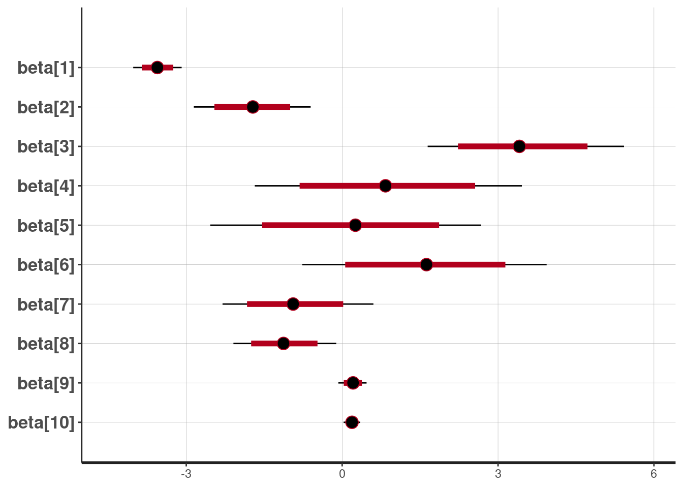

and for $\lambda$ and ${\sigma }^2$

plot(fit, pars = c("lambda", "sigma2"))

ci_level: 0.8 (80% intervals)

outer_level: 0.95 (95% intervals)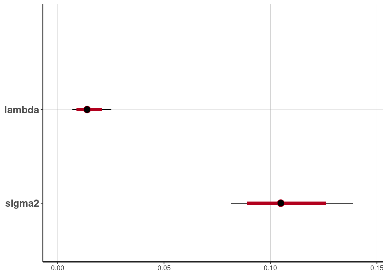

Extract the draws for $\lambda$ and ${\sigma }^2$ and plot histograms.

postsamples <- extract(fit, pars = c("lambda", "sigma2"))
par(mfrow = c(1,2))
hist(postsamples$lambda, 50, freq = FALSE, col = colors[2], 
     xlab = expression(lambda), ylab = "posterior density", 
     main = expression(lambda))
hist(sqrt(postsamples$sigma2), 50, freq = FALSE, col = colors[2], 
     xlab = expression(sigma), ylab = "posterior density",
     main = expression(sigma))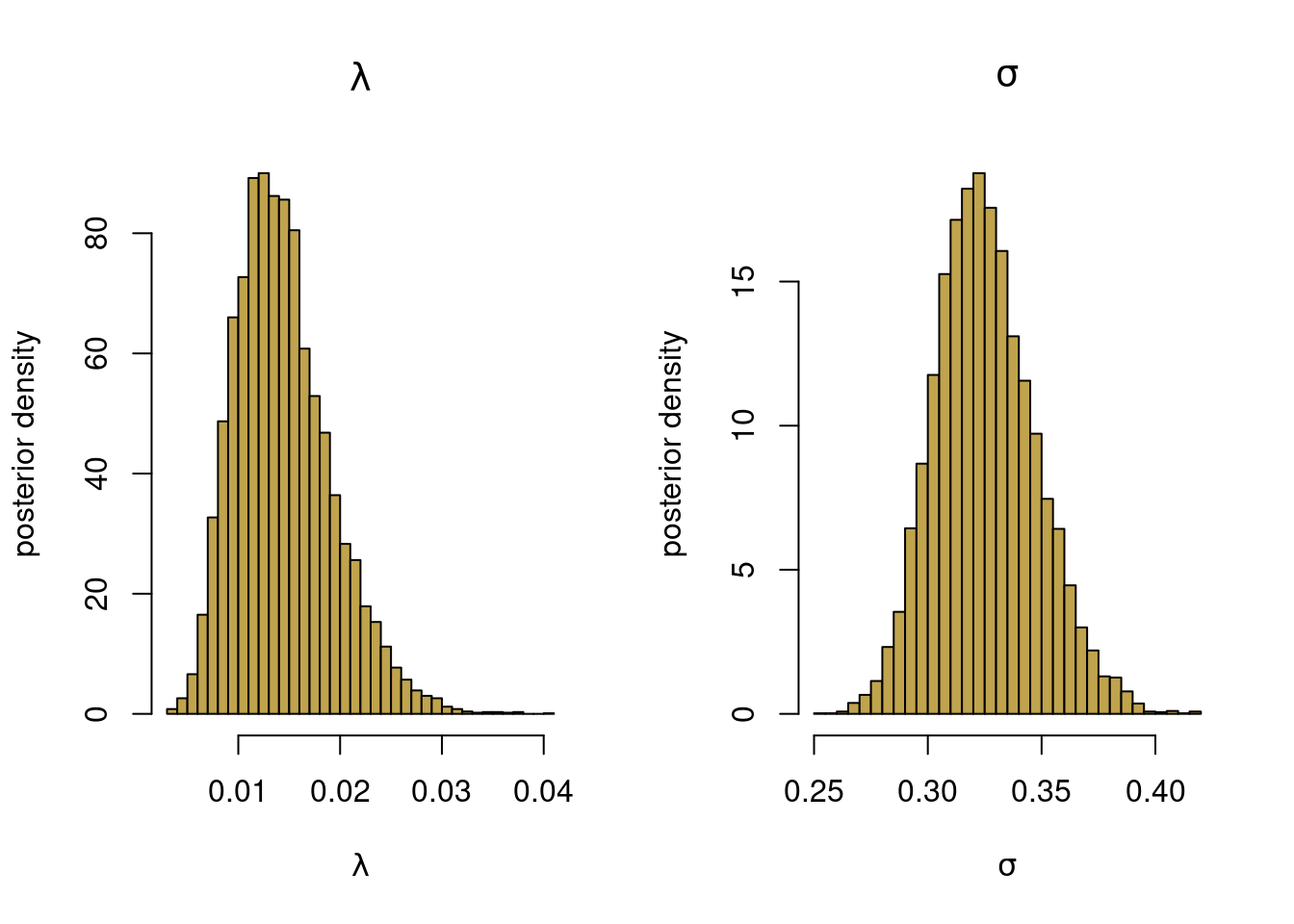

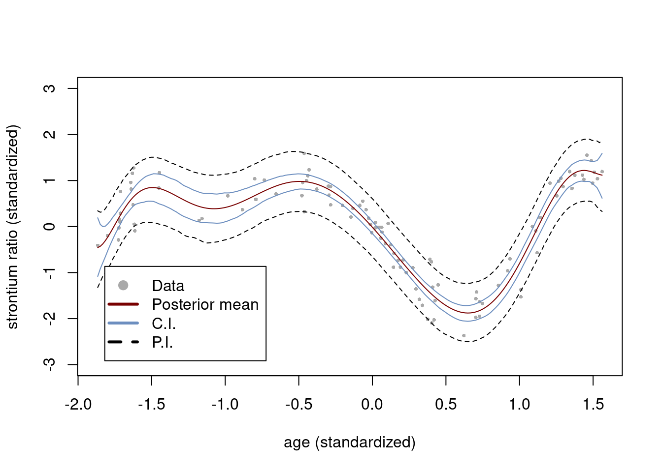
Plot the fit with 95% credible bands

nThin = 10  # Only keep every nThin draws (for storage)
m = floor(nDraws/nThin)
nGrid <- 200 # Number of gridpoints in x-space
postsamples <- extract(fit)
nDraws <- dim(postsamples$beta)[1]
xGrid <- seq(min(x), max(x), length = nGrid)
XGrid = matrix(rep(0, nGrid*degree), nGrid, degree)
for (k in 1:degree){
  XGrid[, k] = xGrid^k
}
postSampRegLine <- matrix(rep(0, m*length(xGrid)), m, length(xGrid))
predSamp <- matrix(rep(0, m*length(xGrid)), m, length(xGrid))
for (i in 1:m){
  j = 1 + (i-1)*nThin
  postSampRegLine[i,] <- postsamples$beta0[j] + XGrid %*% postsamples$beta[j,]
  predSamp[i,] <- postSampRegLine[i,] + rnorm(1, 0, sqrt(postsamples$sigma2[i]))
}
plot(x, y, pch = 16, col = "darkgray", cex = 0.5, ylim = c(-3,3),
     xlab = "age (standardized)", ylab = "strontium ratio (standardized)")
lines(xGrid, colMeans(postSampRegLine), type = "l", col = colors[3])
lines(xGrid, apply(postSampRegLine, 2, quantile, probs = c(0.025) ), type = "l", col = colors[1])
lines(xGrid, apply(postSampRegLine, 2, quantile, probs = c(0.975) ), type = "l", col = colors[1])
lines(xGrid, apply(predSamp, 2, quantile, probs = c(0.025) ), type = "l", lty = 2, col = "black")
lines(xGrid, apply(predSamp, 2, quantile, probs = c(0.975) ), type = "l", lty = 2, col =  "black")

legend(x = "bottomleft", inset=.05,
         legend = c("Data", "Posterior mean", "C.I.", "P.I."), lwd = c(3,3,3,3),
         pch = c(19,NA,NA,NA), lty = c(0,1,1,2),
         col = c("darkgray", colors[3], colors[1], "black"), box.lty=1
  )

Footnotes

1. Chaudhuri, P. and J. S. Marron (1999). Sizer for exploration of structures in curves. Journal of the American Statistical Association