# install.packages("mvtnorm")
# install.packages("RColorBrewer")
library(mvtnorm) # package with multivariate normal density
library(RColorBrewer) # just some fancy colors for plotting
prettyCol = brewer.pal(10,"Paired")Posterior approximation - logistic regression
Load packages
Settings
chooseCov <- c(1:16) # covariates to include in the model
tau <- 10;           # Prior std beta~N(0,tau^2*I)
Reading data and setting up the prior
Data<-read.table("https://raw.githubusercontent.com/mattiasvillani/BayesLearnCourse/master/Notebooks/R/SpamReduced.dat",header=TRUE) # Reduced spambase data (http://archive.ics.uci.edu/ml/datasets/Spambase/)
covNames <- names(Data)[2:length(names(Data))]; # Read off the covariate names
y <- as.vector(Data[,1]);
X <- as.matrix(Data[,2:17]);
X <- X[,chooseCov];                             # Pick out the chosen covariates
covNames <- covNames[chooseCov];                # ... and their names
nPara <- dim(X)[2];

# Setting up the prior
mu <- as.vector(rep(0,nPara)) # Prior mean vector
Sigma <- tau^2*diag(nPara);
Coding up the log posterior function
LogPostLogistic <- function(betaVect,y,X,mu,Sigma){
  nPara <- length(betaVect);
  linPred <- X%*%betaVect;
  logLik <- sum( linPred*y -log(1 + exp(linPred)));
  logPrior <- dmvnorm(betaVect, matrix(0,nPara,1), Sigma, log=TRUE);
  return(logLik + logPrior)
}
Finding the mode and observed information using optim
initVal <- as.vector(rep(0,nPara));
OptimResults<-optim(initVal,LogPostLogistic,gr=NULL,y,X,mu,Sigma,
  method=c("BFGS"), control=list(fnscale=-1),hessian=TRUE)
postMode = OptimResults$par
postCov = -solve(OptimResults$hessian) # inv(J) - Approx posterior covariance matrix
postStd <- sqrt(diag(postCov)) # Computing approximate stdev
names(postMode) <- covNames      # Naming the coefficient by covariates
names(postStd) <- covNames # Naming the coefficient by covariates
The posterior mode is
print(postMode) our over remove internet free
0.4182337582 1.1753728476 2.9209159589 0.9696191548 1.2944179828
hpl X. X..1 CapRunMax CapRunTotal
-1.3114765304 0.5673271835 8.2721841199 0.0118045995 0.0005570864
const hp george X1999 re
-1.4278739763 -2.0411544503 -6.0021765135 -0.4565997686 -0.8577822552
edu
-1.6854611460 The posterior standard deviations are computed from the covariance
print(postStd) our over remove internet free hpl
0.0730320059 0.2321086478 0.3302456199 0.1671111765 0.1412670451 0.4017479109
X. X..1 CapRunMax CapRunTotal const hp
0.0947016268 0.6851475429 0.0017545736 0.0001418867 0.0847302222 0.2998192165
george X1999 re edu
1.1494146395 0.1902088194 0.1476136565 0.2554459768 Plot the marginal posterior of \(\beta\) for the free and hpl covariates
par(mfrow=c(1,2))
gridVals = seq(postMode['free']-3*postStd['free'], postMode['free']+3*postStd['free'],
               length = 100)
plot(gridVals, dnorm(gridVals, mean = postMode['free'], sd = postStd['free']),
     xlab = expression(beta), ylab= "posterior density", type ="l", bty = "n",
     lwd = 2, col = prettyCol[2], main = expression(beta[free]))
gridVals = seq(postMode['hpl']-3*postStd['hpl'], postMode['hpl']+3*postStd['hpl'],
               length = 100)
plot(gridVals, dnorm(gridVals, mean = postMode['hpl'], sd = postStd['hpl']),
     xlab = expression(beta), ylab= "posterior density", type ="l", bty = "n",
     lwd = 2, col = prettyCol[2], main = expression(beta[hpl]))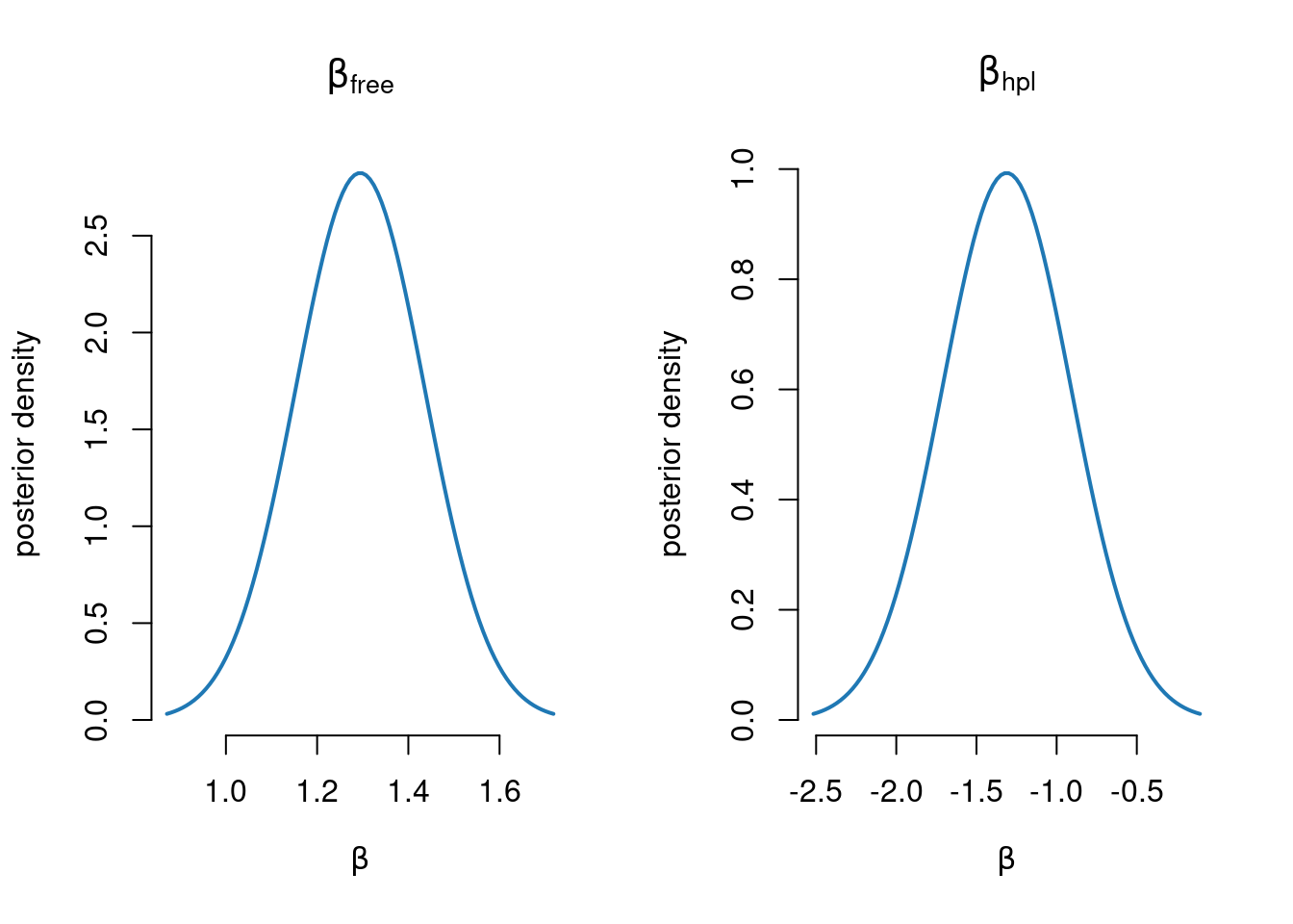
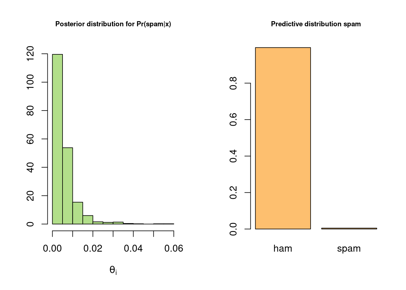
Simulate from normal approximation and make prediction at mean covariate
xStar = colMeans(X)
nSim = 1000
probSpam = rep(0,nSim)
spamPred = rep(0,nSim)
for (i in 1:nSim){
  betaDraw = as.vector(rmvnorm(1, postMode, postCov)) # Simulate a beta draw from approx post
  linPred = t(xStar)%*%betaDraw
  probSpam[i] = exp(linPred)/(1+exp(linPred)) # draw from posterior of Pr(spam|x)
  spamPred[i] = rbinom(n=1,size=1,probSpam[i]) # draw from model given probSpam[i]
}
par(mfrow=c(1,2))
hist(probSpam, freq = FALSE, xlab = expression(theta[i]), ylab= "", col = prettyCol[3],
     main = "Posterior distribution for Pr(spam|x)", cex.main = 0.7)
barplot(c(sum(spamPred==0),sum(spamPred==1))/nSim, names.arg  = c("ham","spam"), col = prettyCol[7],
     main = "Predictive distribution spam", cex.main = 0.7)