Bayesian logistic regression for the Titanic data

Load packages

library(mvtnorm)      # package with multivariate normal density
library(latex2exp)    # latex maths in plots

Settings

tau <- 10             # Prior std beta~N(0,tau^2*I)

Read data and set up prior

df <- read.csv(
  "https://github.com/mattiasvillani/introbayes/raw/main/data/titanic.csv", 
  header=TRUE) 
y <- as.vector(df[,1])
X <- df[,c(5, 4, 2)]
X[, 2] <- 1*(X[,2] == "female")
X[, 3] <- 1*(X[,3] == 1)
X <- as.matrix(cbind(1,X))
p <- dim(X)[2]
varNames = c("intercept", "age", "sex", "firstclass")

# Setting up the prior
mu <- as.vector(rep(0,p)) # Prior mean vector
Sigma <- tau^2*diag(p)

Coding up the log posterior function

LogPostLogistic <- function(betaVect, y, X, mu, Sigma){
  p <- length(betaVect)
  linPred <- X%*%betaVect
  logLik <- sum( linPred*y - log(1 + exp(linPred)))
  logPrior <- dmvnorm(betaVect, matrix(0,p,1), Sigma, log=TRUE)
  return(logLik + logPrior)
}

Finding the mode and observed information using optim

initVal <- as.vector(rep(0,p)); 
OptimResults<-optim(initVal, LogPostLogistic, gr=NULL, y, X, mu, Sigma,
  method = c("BFGS"), control=list(fnscale=-1), hessian=TRUE)
postMode = OptimResults$par
postCov = -solve(OptimResults$hessian) # inv(J) - Approx posterior covar matrix
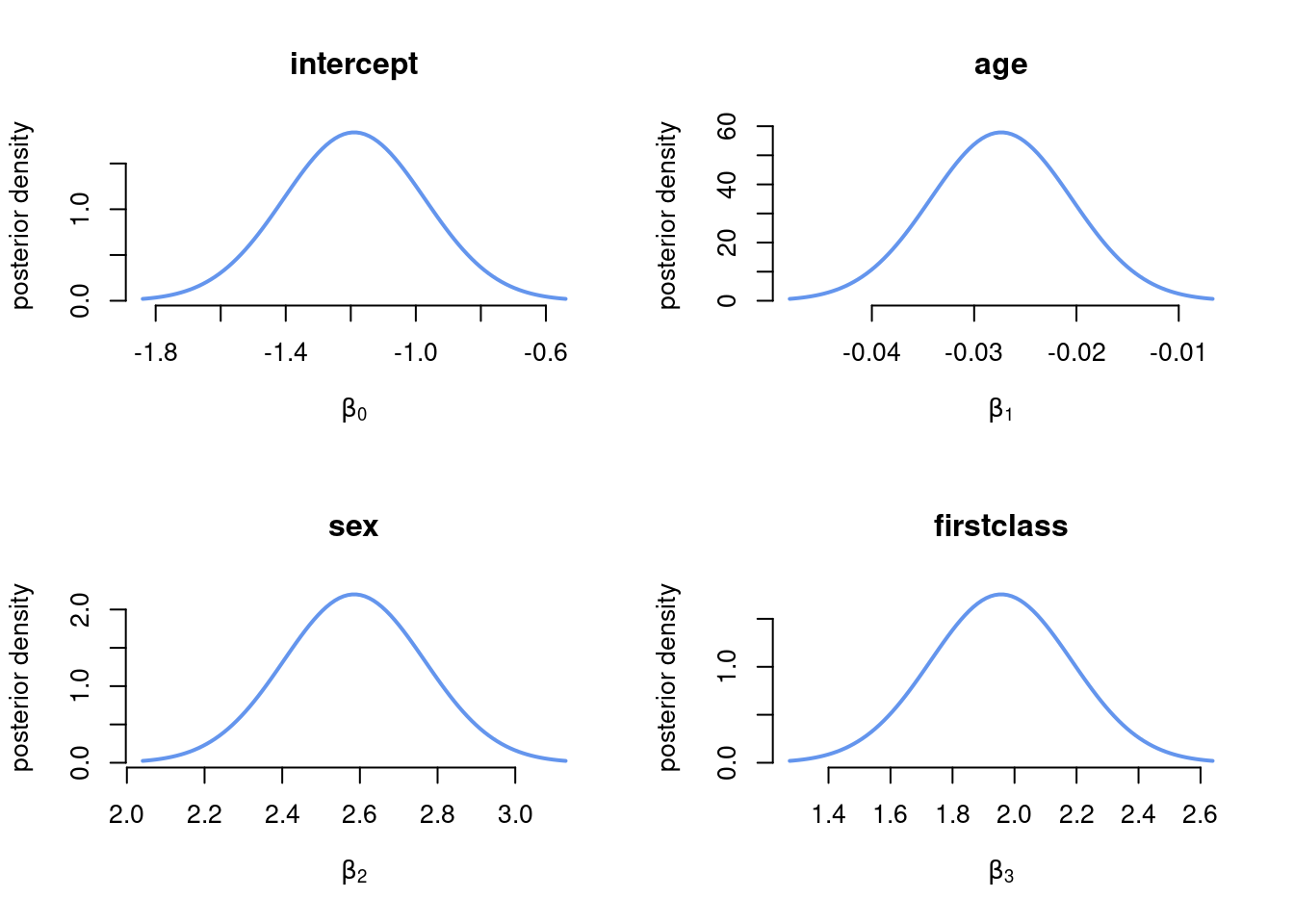
postStd <- sqrt(diag(postCov))         # Approximate stdev

Plot the marginal posterior of $\beta$

Since we have approximated the joint posterior $\mathit{\beta }$ as multivariate normal, the marginal posterior for each ${\beta }_j$ is univariate normal.

par(mfrow=c(2,2))
for (j in 1:4){
  gridVals = seq(postMode[j] - 3*postStd[j], postMode[j] + 3*postStd[j], 
                 length = 100)
  plot(gridVals, dnorm(gridVals, mean = postMode[j], sd = postStd[j]), 
    xlab = TeX(sprintf(r'($\beta_%d$)', j-1)), ylab= "posterior density", 
    type ="l", bty = "n", lwd = 2, col = "cornflowerblue", main =varNames[j])
}

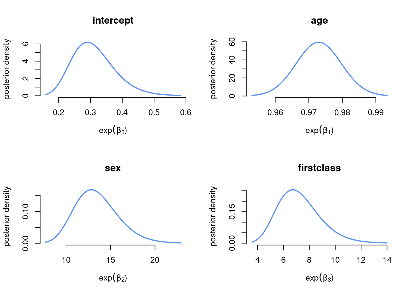
Plot the marginal posterior of the odds $\exp (\beta )$

Since the marginal posterior for each ${\beta }_j$ is approximated as normal, the approximate posterior distribution for the odds $\exp ({\beta }_j)$ is log-normal.

par(mfrow=c(2,2)) 
for (j in 1:4){
  gridVals = exp(seq(postMode[j] - 3*postStd[j], postMode[j] + 3*postStd[j], 
                     length = 100))
  plot(gridVals, dlnorm(gridVals, meanlog = postMode[j], sdlog = postStd[j]), 
    xlab = TeX(sprintf(r'($\exp(\beta_%d$))', j-1)), ylab= "posterior density", 
    type ="l", bty = "n",  lwd = 2, col = "cornflowerblue", main = varNames[j])
}